Case Study 3: Dynamical Properties: The Self-Diffusion Coefficient

This Case Study combines elements of Case Studies 5 and 6 in F&S, which are unfortunately incomplete in their description. The purpose of this Case Study is to demonstrate how one computes a self-diffusion coefficient, $\mathscr{D}$, from an MD simulation of a simple Lennard-Jones liquid. There are two means to computing $\mathscr{D}$: (1) the mean-squared displacement $\left<r^2\right>(t)$, and (2) the velocity autocorrelation function, ${\rm VACF}(t)$.

The self-diffusion coefficient governs the evolution of concentration, $c$, (or number density) according to a generalized transport equation:

$$\frac{\partial c}{\partial t} = \mathscr{D}\nabla^2c$$ (155)

Einstein showed (details in text) that $\mathscr{D}$ is related to the mean-squared displacement, $\left<r^2\right>$:

$$\frac{\partial\left<r^2\right>}{\partial t} = 6\mathscr{D}$$ (156)

At long times, $\mathscr{D}$ should be independent of time; hence

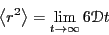$$\left<r^2\right> = \lim_{t\rightarrow\infty}6\mathscr{D}t$$ (157)

We can compute $\left<r^2\right>$, and therefore estimate $\mathscr{D}$, easily using MD simulation. There is, however, a very important consideration concerning periodic boundary conditions. Recall that, during integration, immediately after the position update, we test to see if the update has taken the particle outside of the primary box. If it has, we simply shift the particle's position by a box length in the appropriate dimension and direction. The displacement of the particle during this step is not a box length, but if you consider just the coordinates as they appear in the output, you would think that it is. It is therefore important that we work with unfolded coordinates when computing mean-squared displacement. This is not adequately explained in the text, so we cover it in some detail here.

``Unfolding'' coordinates in a simulation with periodic boundaries requires that we keep track of how many times each particle has crossed a boundary. The code mdlj.c was just modified to allow output of unfolded coordinates in the sample configurations. Here is how it works. In the integration loop, you may recall that the first step is the update of positions (below we consider the $x$-coordinate only):

      rx[i]+=vx[i]*dt+0.5*dt2*fx[i];

The quantity $v_{x,i}\delta t + 1/2\left(\delta t\right)^2f_{x,i}$ is the $x$-displacement of particle $i$ in one time step of length $\delta t$. Now, this displacement may have resulted in a new $x$-coordinate of particle $i$ which is less than zero or greater than the box length $L$, in which case, we shift the coordinate to keep it between 0 and $L$. In addition to performing this shift, we now increment a counter for particle $i$:

      if (rx[i]<0.0) { rx[i]+=L; ix[i]--; }
      if (rx[i]>L)   { rx[i]-=L; ix[i]++; }

The counter ix[i] is incremented by 1 if the $x$-coordinate update takes the particle through the $+x$ boundary, and is decremented by 1 if the update takes the particle through the $-x$ boundary. This counter tells us how box lengths the total $x$-displacement of particle $i$ has accumulated, and its sign gives us the sense of this accumulation. Now, the array rx[] always contains the periodically shifted coordinates, but we can easily generate the unfolded coordinates at any time (say, upon output) by performing the following operation:

       rxu = rx[i]+ix[i]*L;

Here, $L$ is the box length (assumed cubic). In the newly updated code mdlj.c, the integrator and output functions have been modified to allow output of the unfolded coordinates if the user includes the -uf flag on the command line.

Let us now run mdlj using the final configuration from one of the previous runs in the previous case study as an initial state, with the goal of computing $\left<r^2\right>$. (Note that we must still specify $N$ and $rho$ on the command line.) We will go for as much detail as possible, and output the configuration every time step. To limit the amount of data, we will terminate this simulation at 1000 steps. This results in 1,000 xyz data files containing unfolded coordinates. Now, the program msd.c will read all of these configurations in at once (that is, it reads in the entire trajectory), and compute the mean-squared displacement, $\left<r^2\right>$, from this data using a conventional, straightforward algorithm.

The C-code for this algorithm appears below. $M$ is the number of ``frames'' in the trajectory, and $N$ is the number of particles. $\left<r^2\right>(t)$ is computed by considering the change in particle position over an interval of size $t$. Any frame in the trajectory can be considered an origin for any interval size, provided enough frames come after it in the trajectory. This means that we additionally average over all possible time origins. dt is a variable that loops over allowed time intervals. cnt[] counts the number of time origins for a given interval. sdx[] is the array in which we accumulate squared displacement in the $x$-displacements, and has $M$ elements, one for each allowed interval value, including interval length 0.

  for (t=0;t<M;t++) {                // Loop over all frames
    for (dt=1;(t+dt)<M;dt++) {       // Loop over all allowed origins
      cnt[dt]++;                     // Increment the number of origins
      for (i=0;i<N;i++) {
	sdx[dt] += (rx[t+dt][i] - rx[t][i])*(rx[t+dt][i] - rx[t][i]);
	sdy[dt] += (ry[t+dt][i] - ry[t][i])*(ry[t+dt][i] - ry[t][i]);
	sdz[dt] += (rz[t+dt][i] - rz[t][i])*(rz[t+dt][i] - rz[t][i]);
      }
    }
  }

The code fragment below completes the averaging, and outputs the three components of the mean-squared displacement, as well as the total mean-squared displacement.

  for (t=0;t<M;t++) {
    sdx[t] /= cnt[t]?(N*cnt[t]):1;
    sdy[t] /= cnt[t]?(N*cnt[t]):1;
    sdz[t] /= cnt[t]?(N*cnt[t]):1;
    fprintf(stdout,"%.5lf %.8lf %.8lf %.8lf %.8lf"
	    t*step*md_time_step,sdx[t],sdy[t],sdz[t],
	    sdx[t]+sdy[t]+sdz[t]);
  }

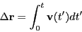
Below is a plot of mean-squared displacement from a simulation of 1,000 steps. Recall that the Einstein relation holds as $t\rightarrow\infty$. We see in this plot that, for low times, $\left<r^2\right> \propto t^2$, which indicates that motion in this regime is not diffusive; it is in fact ballistic. This ballistic behavior becomes apparently diffusive at a time around 0.1 $\tau$. Considering the data beyond $t > 0.1$, we can roughly estimate $\mathscr{D}$ at about 0.06.

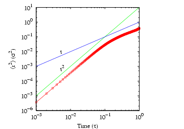Mean-squared displacement in a Lennard-Jones fluid from an MD simulation in which $N$ = 108, $rho$ = 0.8442, sampled every time step for 1,000 steps. Measured temperature $T = 1.20 \pm 0.011$ and pressure, $P = 3.81 \pm 0.11$.. ¹

¹ This graph was produced using gnuplot and a script found here.

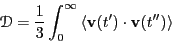
It is advisable, however, to compute $\mathscr{D}$ using much longer-scale data. The ballistic crossover indicates that we need not consider time intervals below 0.1 (100 steps of $\delta t$ = 0.001). In fact, in a long simulation of 600,000 steps, we can get a good estimate of $\mathscr{D}$ by considering samples every 1,000 steps. To obtain a more unambiguous estimate of $\mathscr{D}$, we can plot $\left<r^2\right>/(6t)$ vs $1/t$ and extrapolate to $1/t\rightarrow 0$, where $\left<r^2\right>/(6t) = \mathscr{D}$.

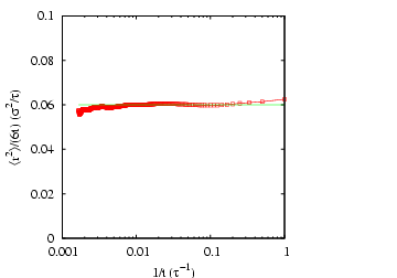Mean-squared displacement in a Lennard-Jones fluid from an MD simulation in which $N$ = 108, $rho$ = 0.8442, sampled every 1,000 time steps for 600,000 steps. The horizontal line indicates that $\mathscr{D}$ = 0.06. Measured temperature $T = 1.215 \pm 0.0006$ and pressure, $P = 3.71 \pm 0.005$. ¹

¹ This graph was produced using gnuplot and a script found here.

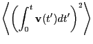
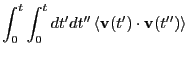
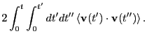
The velocity autocorrelation function route to the diffusion constant begins with the realization that one can reconstruct the displacement of a particle over a time interval $t$ by simply integrating its velocity:

$$\Delta{\bf r} = \int_0^t {\bf v}(t^\prime)dt^\prime$$ (158)

So, the mean squared displacement can be expressed

$$\left<r^2\right> = \left<\left(\int_0^t{\bf v}(t^\prime)dt^\prime\right)^2\right>$$ (159)

$$= \int_0^t\int_0^t dt^\prime dt^{\prime\prime} \left<{\bf v}(t^\prime)\cdot{\bf v}(t^{\prime\prime})\right>$$ (160)

$$= 2\int_0^t\int_0^{t^\prime} dt^\prime dt^{\prime\prime} \left<{\bf v}(t^\prime)\cdot{\bf v}(t^{\prime\prime})\right>.$$ (161)

The third equality arises because we can swap $t^\prime$ and $t^{\prime\prime}$. The quantity $\left<{\bf v}(t^\prime)\cdot{\bf v}(t^{\prime\prime})\right>$ is the velocity autocorrelation function. This is an example of a Green-Kubo relation; that is, a relation between a transport coefficient, and an autocorrelation function of a dynamical variable. Eq. 156 then leads to

$$\mathscr{D} = \frac{1}{3}\int_0^\infty \left<{\bf v}(t^\prime)\cdot{\bf v}(t^{\prime\prime})\right>$$ (162)

So, the second route to computing $\mathscr{D}$ requires that we numerically integrate $\left<{\bf v}(t^\prime)\cdot{\bf v}(t^{\prime\prime})\right>$ out to very large times. How large? First, let's try to understand the behavior of $\left<{\bf v}(t^\prime)\cdot{\bf v}(t^{\prime\prime})\right>$.

In three dimensions, we compute this by computing the components and adding them together, as we did for mean-squared displacement:

$$\left<{\bf v}(t^\prime)\cdot{\bf v}(t^{\prime\prime})\right>... ...rime})\right>+ \left<v_z(t^\prime)v_z(t^{\prime\prime})\right>$$ (163)

Because the system is (nearly) isotropic, we should expect all these components to be equal. The plot of $\left<{\bf v}(0)\cdot{\bf v}(t)\right>$ vs. $t$ shown below indicates the level to which we can expect the three components to be equal for such a small system. This data was computed using the code vacf.c.

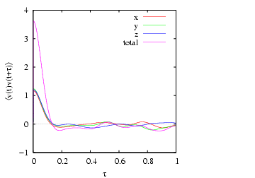Velocity autocorrelation in a Lennard-Jones fluid from an MD simulation in which $N$ = 108, $rho$ = 0.8442, sampled every time step for 1,000 steps. Measured temperature $T = 1.20 \pm 0.011$ and pressure, $P = 3.81 \pm 0.11$. ¹

¹ This graph was produced using gnuplot and a script found here.

Integrating the composite out to $t = 1.0$ gives $\mathscr{D} \approx 0.047$, which is not terribly good compared to $\mathscr{D}$ computed by mean-squared displacement. This is because, although the VACF below about $t = 0.1$ contributes a heavy fraction to the integral, the VACF is a very slowly decaying function, so the tail contributes a significant amount to the integral as well. So, just for fun, I extended the 1,000-step run out to 3,000 steps, then recomputed the VACF. The result: $\mathscr{D} = 0.043.$ This result is no better, and this shows that it is often difficult to get reliable estimates of transport coefficients from Green-Kubo-type relations without including much longer-time contributions. This conventional algorithm for computing the VACF becomes quite costly as we increase the the run time; it scales like $t^2$. For this reason, it is often desirable to use more sophisticated sampling techniques when estimating transport coefficients using Green-Kubo-type analyses. In the interest of time, we won't consider these techniques in this course.