The Nosé-Hoover Chain

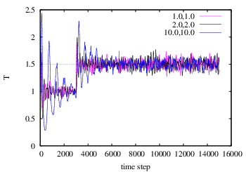
The final thermostat we consider is one based on the extended Lagrangian formalism, which leads to a deterministic trajectory; i.e., there are no random forces or velocities to deal with. The most common and so far most reliable thermostat of this kind is the Nosé-Hoover thermostat. This thermostat can be implemented as a ``single'' or a ``chain''; here, we consider a chain.

The basic idea of the Nosé-Hoover thermostat is to use a friction factor to control particle velocities. This friction factor is actually the scaled velocity, $v_{\xi_1}$, of an additional and dimensionless degree of freedom, $\xi_1$. This degree of freedom has an associated ``mass'', $Q_1$, which effectively determines the strength of the thermostat. The equations of motion obeyed by this additional degree of freedom guarantee that the original degrees of freedom (${\bf r}^N$, ${\bf p}^N$) sample a canonical ensemble. This degree of freedom is the terminus of a chain of similar degrees of freedom, each with their own mass. The chain has a total of $M$ ``links.'' The overall set of equations of motion are:

$$\dot{\bf r}_i = \frac{\dot{\bf p}_i}{m_i}$$ (190)

$$\dot{\bf p}_i = {\bf F}_i - \frac{p_{\xi_1}}{Q_1}{\bf p}_i$$ (191)

$$\dot{\xi}_k = \frac{p_{\xi_k}}{Q_k} k = 1,\dots,M$$ (192)

$$\dot{p_{\xi_1}} = \left(\sum_i\frac{p_i^2}{m_i} - Lk_BT\right)-\frac{p_{\xi,2}}{Q_2}p_{\xi_1}$$ (193)

$$\dot{p_{\xi_k}} = \left(\frac{p^2_{\xi_{k-1}}}{Q_{k-1}} - k_BT\right) - \frac{p_{\xi_{k+1}}}{Q_{k+1}}p_{\xi_k}$$ (194)

$$\dot{p_{\xi_k}} = \left(\frac{p^2_{\xi_{M-1}}}{Q_{M-1}} - k_BT\right)$$ (195)

The main advantage of the Nosé-Hoover chain thermostat is that the dynamics of all degrees of freedom are deterministic and time-reversible. No random numbers are used. The code mdlj_nhc.c implements an $M$ = 2 Nosé-Hoover chain thermostat in an MD simulation of an Lennard-Jones fluid, by implementing Algorithms 30, 31, and 32 from F&S. The two masses of the thermostats are defaulted to $Q_1$ = $Q_2$ = 0.1. This ``low'' mass results in a ``loose'' control of temperature; higher masses mean a tighter control. $\xi_1$ is the degree of freedom whose velocity is used to scale particle velocities, so one might hypothesize that the mass $Q_1$ is the more important. (You can verify this as an exercise.) Though I haven't verified that my code is 100% bug-free, apparently, the effect of increasing the mass of the coupling degree of freedom is to lengthen the decay time constant of the response to an instantaneous temperature jump:

Instantaneous temperature, $T$, vs. time in an MD simulation of 256 particles at a density of 0.8442, with temperature controlled by a chain of two Nosé-Hoover thermostats, for various values of the masses $Q_1$ and $Q_2$.

If anyone finds a bug in this code, I will buy you a refreshing beverage of your choice.