Thermodynamic Integration

Thermodynamic integration is a conceptually simple, albeit expensive, way to calculate free energy differences from MC or MD simulations. In this example, we will consider the calculation (again) of chemical potential in a Lennard-Jones fluid at a given temperature and density, a task performed very well already by the Widom method (so long as the densities are not too high.) More details of the method can be found in Reference [15].

We begin with the relation derived in the book for a free energy difference, $F_{II} - F_{I}$, between two systems which are identical (same number of particles, density, temperature, etc.) except that they obey two different potentials. System I obeys $\mathscr{U}_I$ and System II $\mathscr{U}_{II}$. To measure this free energy difference, we must integrate along a reversible path from I to II. So let us suppose that we can write a ``metapotential'' that uses a switching parameter, $\lambda$, to measure distance along this path. So, when $\lambda = 0$, we are in System I, and when $\lambda = 1$ we are in System II. One way we might encode this (though this is not necessarily a general splitting, as we shall see below) is

$$\mathscr{U}\left(\lambda\right) = \left(1-\lambda\right)\mathscr{U}_{I} + \lambda\mathscr{U}_{II}$$ (210)

Let us consider the canonical partition function for a system obeying a general potential $\mathscr{U}\left(\lambda\right)$:

$$Q\left(N,V,T,\lambda\right) = \frac{1}{\Lambda^{3N}N!}\int d{\bf r}^N\exp\left[-\beta\mathscr{U}\left(\lambda\right)\right]$$ (211)

Recalling that the free energy is given by $F = -k_BT\ln Q$, we can express the derivative of the Helmholtz free energy with respect to $\lambda$:

$$\left(\frac{\partial F\left(\lambda\right)}{\partial\lambda}\right)_{N,V,T} = -\frac{1}{\beta}\frac{\partial}{\partial\lambda}\ln Q\left(N,V,T,\lambda\right)$$ (212)

$$= -\frac{1}{\beta Q\left(N,V,T,\lambda\right)}\frac{\partial Q\left(N,V,T,\lambda\right)}{\partial\lambda}$$ (213)

$$= \frac{ \begin{minipage}{6cm} \begin{displaymath} \int d{\bf r}^N ... ...t[-\beta\mathscr{U}\left(\lambda\right)\right] \end{displaymath}\end{minipage}}$$ (214)

The free energy difference between I and II is given by:

$$F_{II} - F{I} = \int_{\lambda=0}^{\lambda=1}\left<\frac{\partial\mathscr{U}}{\partial\lambda}\right>_\lambda d\lambda$$ (215)

where, $\left<\frac{\partial\mathscr{U}}{\partial\lambda}\right>_\lambda$ is the ensemble average of the derivative of $\mathscr{U}$ with respect to $\lambda$.

To compute $\mu_{\rm ex}$, we imagine two systems: System I has $N-1$ ``real'' particles, and 1 ideal gas particle, and system II has $N$ real particles. The two free energies can be written:

$$F_{\rm I} = F_{\rm id}\left(N,V,T\right) + F_{\rm ex}\left(N-1,V,T\right)$$ (216)

$$F_{\rm II} = F_{\rm id}\left(N,V,T\right) + F_{\rm ex}\left(N,V,T\right)$$ (217)

For large values of $N$, we see that $\mu_{\rm ex} = F_{\rm II} - F_{\rm I}$. So, we have another route to compute $\mu_{\rm ex}$. First, we tag a particle $i_\lambda$, call it the ``$\lambda$-particle'', and apply the following modified potential to its pairwise interactions:

$$U_{\rm LJ,\lambda}\left(r;\lambda\right) = 4\left(\lambda^5r^{-12} - \lambda^3r^{-6}\right)$$ (218)

So, the total potential is given by

$$\mathscr{U} = {\sum_{i<j}} ^\prime U_{\rm LJ}\left(r_{ij}\ri... ... \sum_i U_{\rm LJ,\lambda}\left(r_{i,i_\lambda};\lambda\right)$$ (219)

where the prime denotes that we ignore particle $i_\lambda$ in the sum. When $\lambda = 1$, all particles interact fully, and we have System II.

Next, we conduct many independent MC simulations at various values of $\lambda$ and a given value of $rho$ and $T$, generating for each $\left(T,\rho\right)$ a table of $\left<\partial\mathscr{U}/\partial\lambda\right>_\lambda$ vs. $\lambda$ which can be integrated to yield a single value for $\mu_{\rm ex}$. This turns out to be an expensive way to compute the chemical potential for a Lennard-Jones fluid, compared to the Widom method (Sec. 6.1), for at least low to moderate densities.

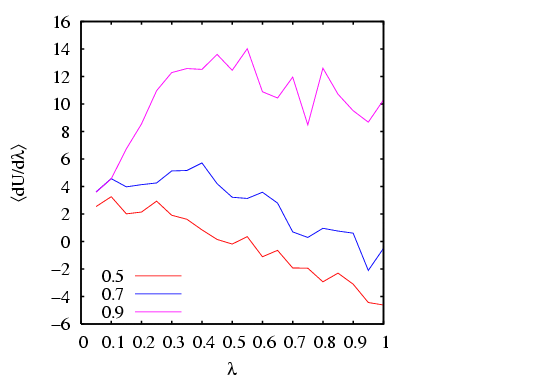
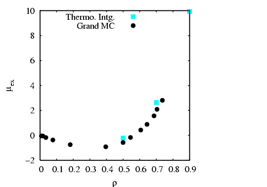
I have done a rough comparison of the thermodynamic integration method described above to the grand canonical MC simulation technique described in Sec. 5.1. Below is a plot of $\left<\partial\mathscr{U}/\partial\lambda\right>_\lambda$ vs. $\lambda$ for three densities $\rho \in \left\{0.5, 0.7, 0.9\right\}$. Each point is computed from a single MC simulation using the code mclj_ti.c. The temperature was $T$ = 2.0, and run for 10$^6$ cycles for $N$ = 216. We see that the data is not terribly smooth; it is not clear how many more cycles would result in smoother data.

$\left<\partial\mathscr{U}/\partial\lambda\right>_\lambda$ vs. $\lambda$ for the Lennard-Jones fluid for three values of $rho$ at $T$ = 2.0, computed from MC simulations of 216 particles for 10$^6$ cycles.

However, integration is not too sensitive to these fluctuations. As we see below, integrating each of these curves to produce a single value of $\mu_{\rm ex}$ produces values that are not too off from the grand canonical simulations.

$\left<\partial\mathscr{U}/\partial\lambda\right>_\lambda$ vs. $\lambda$ for the Lennard-Jones fluid for three values of $rho$ at $T$ = 2.0, computed from MC simulations of 216 particles for 10$^6$ cycles.

The grand canonical simulations are of course much cheaper, as it requires only a single MC simulation to give a value of $\mu_{\rm ex}$. However, thermodynamic integration is a generally applicable technique for computing free energy differences.

Questions:

1. Can we make the agreement better by running more MC cycles? How about by using more values of $\lambda$?
2. How does this compare to the Widom method?