


Next: Monte Carlo Simulation
Up: Statistical Mechanics: A Brief
Previous: Entropy and Temperature
Section 2.2 of Frenkel & Smit [1] discusses a
derivation of the ``quasi-classical'' representation of the canonical
partition function,
 :
:
![\begin{displaymath}
Q_{\rm classical} = \frac{1}{h^{dN}N!}\int \int d{\bf r}^N d...
...\left[-\beta\mathscr{H}\left({\bf r}^N,{\bf p}^N\right)\right]
\end{displaymath}](img153.png) |
(42) |
 is the Hamiltonian
function which computes the energy of a point in phase space. The
derivation of Eq. 42 is not repeated here. What is
important is that the probability of a point in phase space is
represented as
is the Hamiltonian
function which computes the energy of a point in phase space. The
derivation of Eq. 42 is not repeated here. What is
important is that the probability of a point in phase space is
represented as
![\begin{displaymath}
P\left({\bf r}^N,{\bf p}^N\right) = \left(Q_{\rm classical}\...
...left[-\beta\mathscr{H}\left({\bf r}^N,{\bf p}^N\right)\right].
\end{displaymath}](img155.png) |
(43) |
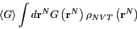
So, the general ``sum-over-states' ensemble average of quantum
statistical mechanics, first presented in
Eq. 1, becomes an integral over phase space in
classical statistical mechanics:
![\begin{displaymath}
\left<G\right> = \frac{
\mbox{
\begin{minipage}{8cm}
\beg...
...,{\bf p}^N\right)\right]
\end{displaymath} \end{minipage} }},
\end{displaymath}](img156.png) |
(44) |
where
 is the value of the
observable
is the value of the
observable  at phase space point
 . Before moving on, it is useful to recognize that
we normall simplify this ensemble average by noting that, for a
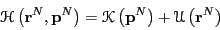
system of classical particles, the usual choice for the Hamiltonian
has the form
. Before moving on, it is useful to recognize that
we normall simplify this ensemble average by noting that, for a
system of classical particles, the usual choice for the Hamiltonian
has the form
 |
(45) |
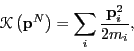
where  is the kinetic energy, which is only a function of
momenta, and
is the kinetic energy, which is only a function of
momenta, and  is the potential energy, which is only a
function of position. The canonical partition function,
is the potential energy, which is only a
function of position. The canonical partition function,  , can in
this case be factorized:
, can in
this case be factorized:
The quantity in the left-hand braces is the ideal gas partition
function, because it corresponds to the case when the potential
is 0. (Note that we have multiplied and divided by
 ; this is the equivalent of scaling the positions in the
integration over positions.) The quantity in the right-hand braces
is called the configurational partition function,
; this is the equivalent of scaling the positions in the
integration over positions.) The quantity in the right-hand braces
is called the configurational partition function,  .
.
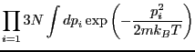
Because the kinetic energy has the simple form,
 |
(49) |
where  is the mass of particle
  , the integral over particle
momenta can be evaluated analytically:
, the integral over particle
momenta can be evaluated analytically:
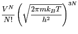
(We have assumed all particles have the same mass,  ; in the case
of distinct masses, this is just a product of similar factors.)
; in the case
of distinct masses, this is just a product of similar factors.)
 becomes
where  is the de Broglie wavelength.
So, when the observable is a function of positions only, the
ensemble average becomes a configurational average:
![\begin{displaymath}
\left<G\right> = Z^{-1}\int d{\bf r}^N \exp\left[-\beta\mathscr{U}\left({\bf r}^N\right)\right] G\left({\bf r}^N\right).
\end{displaymath}](img179.png) |
(54) |
Note that the integation over momentum yields a factor in
both the numerator and denominator, and thus divides out. We can write
this configurational average using a probability distribution,  ,
as
,
as
 |
(55) |
where
 |
(56) |
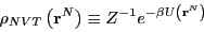
is called the ``canonical probability distribution.'' As pointed out
on p. 15 of Frenkel & Smit [1],
Eq. 54 is ``the starting point for virtually all
classical simulations of many-body systems''; that is, it is the
starting point for all simulations discussed in this course.
Next: Monte Carlo Simulation
Up: Statistical Mechanics: A Brief
Previous: Entropy and Temperature
cfa22@drexel.edu
![$\displaystyle \int d{\bf p}^N \exp\left[-\beta\mathscr{K}\left({\bf p}^N\right)\right]$](img170.png)
![$\displaystyle \frac{V^N}{N!h^{3N}} \int d{\bf p}^N \exp\left[-\beta\mathscr{K}\left({\bf p}^N\right)\right]$](img174.png)

![$\displaystyle \frac{1}{h^{3N}N!} \left\{\int d{\bf p}^N \exp\left[-\beta\mathsc...
...int d{\bf r}^N \exp\left[-\beta\mathscr{U}\left({\bf r}^N\right)\right]\right\}$](img163.png)
![$\displaystyle \left\{\frac{V^N}{h^{3N}N!} \int d{\bf p}^N \exp\left[-\beta\math...
...int d{\bf r}^N \exp\left[-\beta\mathscr{U}\left({\bf r}^N\right)\right]\right\}$](img164.png)