Case Study 3: Hard-Disk Dumbbells in 2D

In this case study, we consider a slightly different system than the hard-disk system in the previous case study. Here, we imagine that pairs of disks are tethered together to form dumbbells. The “bond-length” of a dumbbell is a constant parameter, $r_0$. We will again confine the dumbbells to a circle.

What is new is how we have to consider the trial moves for this system. We cannot simply select a random particle and try to displace it, because this is likely to violate the constant bond-length of the dumbbell that particle belongs to. How then do we generate new configurations? A simple idea is to use two kinds of trial moves, translation of entire dumbbells and rotation of dumbbells around their centers of mass. This was originally presented in Sec. 3.3.3. In order to implement an MC code with more than one trial move, we must include a “trial move selection rule” which randomly selects a trial move based on their user-defined “weights”.

The code hdisk-dumbbells.c implements a MC simulation of hard-disk dumbbells. One specifies a number of particles using -N # at the command line, and the number of dimers is assumed to be $N$/2. One can specify two of $N$, $\rho$ (areal particle density), or $R$ (confining domain diameter). One can also specify $\delta r$ (maximum dimer displacement distance) and $\delta \phi$ (maximum dimer rotation angle), as well as the dimer bond length $r_0$. An XYZ-format trajectory can be saved every -fs cycles using -traj my_traj.xyz.

Let's run this program for $N$ = 200, $\rho$ = 0.6, $\delta r$ = 1, $\delta \phi = \pi$, for 10,000 cycles, saving 1000 snapshots in traj.xyz:

cd
cd cheT580-202035/instructional-codes/my_work
mkdir hddb_run
cd hddb_run
gcc -O3 -o hddb../../originals/hdisk-dumbbells.c -lm -lgsl
./hddb -rho 0.6 -dr 1 -da 3.1 -dw 0.5 -N 200 -traj traj.xyz -fs 10 -nc 10000
# R = 10.30; rho = 0.60; N = 200; r_0 = 1.00; s = 1.00; disp_wt = 0.50, seed = 23410981
Results:
Number of trial moves:             2000000
Maximum displacement length:       1.000
Number of displacement attempts:   999499
Maximum rotation angle (radians):  3.100
Number of rotation attempts:       1000501
Displacement acceptance ratio:     0.344
Rotation acceptance ratio:         0.405
Reject Fraction Out-of-bounds:     0.10037
Reject Fraction Overlap:           0.89963
Trajectory saved to:               traj.xyz
ls
hddb traj.xyz

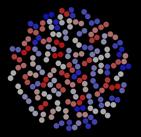
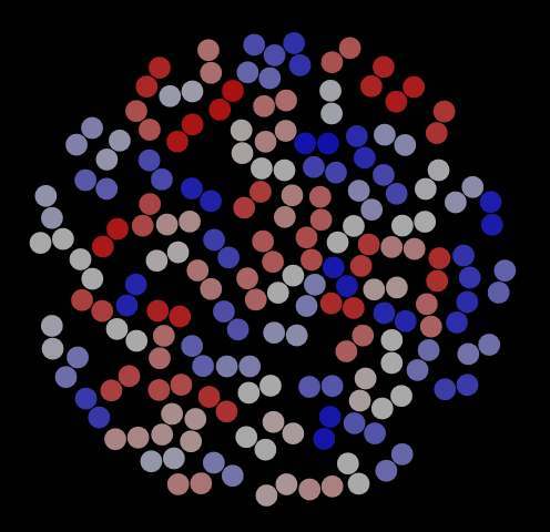
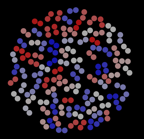
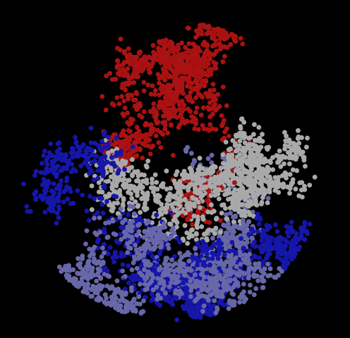
As with the hard disks, we can use VMD to visualize frames in this trajectory. Fig. 8 shows three representative snapshots from this simulation, along with a special view showing the histories of four particular dimers. This last rendering serves to indicate that dimers have mostly explored the entire domain for this number of cycles (is this the case for 1,000 cycles?).

Figure 8: Snapshots from a short hard-disk-dumbbell MC simulation at 0, 5000, and 10,000 cycles. Images were rendered in VMD in an orthographic view along [0,0,-1], and particles were rendered as “points” and colored according to index. Far right: traces of positions of four particular dimers throughout the trajectory.

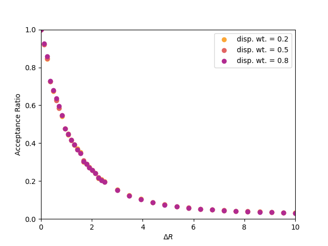
Consider the following question: Does the acceptance ratio of rotational moves depend upon the weight given to displacement moves? Why or why not? Below is a plot of the acceptance ratio vs. the maximum displacement for a system of 100 dumbbells at a density of 0.5, for various displacement move weights between 0.1 and 0.9. As you can see, there appears to be no effect on the acceptance of trial displacements if we change how frequently we perform them relative to trial rotations.

Figure 9: Displacement acceptance ratio vs. maximum dumbbell displacement for various displacement trial move weights between 0.2, 0.5, and 0.8. $N$ = 200 (100 dumbbells), $\rho$ = 0.5, and $R$ = 11.3.

Let's consider computing an observable function that describes how the molecules order themselves in the circular domain. One such meaningful function we'll call $\langle P[\theta(r)]\rangle$, where

$$P(\theta) = \cos^2\theta-\frac{1}{2}$$ (94)

and $\theta$ is defined as the angle between a dumbbell's bond and a vector joining its midpoint to the domain origin. $\langle P[\theta(r)]\rangle$ is therefore the expectation of $P$ averaged over all dumbbells located between $r$ and $r+\delta r$ from the origin. Why is this a meaningful measure of order for this system? Consider that dumbbells near the periphery like to align so their bonds are tangent to the periphery itself and therefore perpendicular to the radius, and the further away from the periphery you look, the less likely this order is to appear. When two vectors are perpendicular, their angle betwen them is $\pi$ and since $\cos\pi=0$, we expect $\langle P\rangle$ to be -0.5. Is this what we observe for our system?

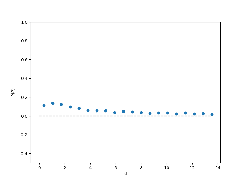
To explore this function, the code hdisk_dumbbells_order.c was copied from hdisk_dumbbells.c. In hdisk_dumbbells_order.c, I introduce the arrays theta[] to hold a tally of $\cos^2\theta$ values and Rcount[] to hold a count of hits in each radial bin, so that $\langle P(\theta(r)) \rangle$ = theta[i]/Rcount[i] - 0.5, where i is the radial bin index set by $R$ and a specified number of bins. Fig. 10 shows $P$ vs $r$ for a hard-disk dumbbell system at density 0.66 with 400 particles (200 dumbbells), run for 500,000 cycles. We can see some interesting structure here, notably that it looks like, on average, there is very little ordering at the periphery and it becomes substatially higher as we get closer to the origin, though still not very strong. Notably, at about 1 $\sigma$ from the periphery, we see a dip in $P$ that might indicate an enrichment in tangentially-oriented dumbbells.

Figure 10: Order parameter $P$ vs radius for a hard-disk dumbbell system confined to a circle of radius 13.9 $\sigma$.

A final note: Since this is a 2D system, we don't use the second Legendre polynomial of $\cos\theta$:

$$P_2(x)=\frac12(3x^2-1)$$ (95)

The reason for this is clear. Suppose $f(\theta)$ is the probability distribution of the angle $\theta$. Now, since the molecules are not polar (they have no head or tail), $\theta$ is meaningful only on the domain $[0,\frac{\pi}{2}]$. Suppose further that there is no preferred angle; i.e., $f$ is a constant. In 2D, normalization requires

$$1=f\int_0^{\pi/2}d\theta \rightarrow f=\frac{2}{\pi},$$ (96)

and in this case, with no preferred orientation, the average of $\cos^2\theta$ is

$$\left<\cos^2\theta\right> = \frac{2}{\pi}\int_0^{\pi/2} \cos^2\theta d\theta = \frac{2}{\pi}\frac{\pi}{4} = \frac12.$$ (97)

And Eq. 95 will have the described behavior. The second Legendre polynomial evaluates to zero when $\cos^2\theta$ is $\frac13$, which is indeed what $\left<\cos^2\theta\right>$ evaluates to when $f$ is a constant in three dimensions.