The Liouville Operator Formalism to Generating MD
Integration Schemes
In this section, we present an elegant formalism for deriving MD
integrators, as discussed by Tuckerman et
al. [6]. What we present here is essentially the
first two parts of the second section of
Reference [6], including some of my own elaboration
and some of that presented in section 4.3 of F&S.
Imagine a quantity  which is a function of particle positions
  and momenta
  . Its time derivative is given by
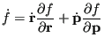 |
(128) |
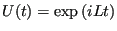
We can write down a formal solution to this equation. First,
define the Liouville operator as
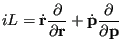 |
(129) |
As Tuckerman points out,
the  is there by convention and ensures that the operator is Hermitian. We can re-express Eq. 128 as
 |
(130) |
which we solve directly to yield
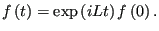 |
(131) |
If is itself a vector quantity identical to the set of positions
and momenta,  , we have a way to express, formally, the
evolution of the system:
, we have a way to express, formally, the
evolution of the system:
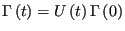 |
(132) |
where
 is the classical propagator.
The idea with numerical integration is that we find a way to represent
the propagator as a discrete algorithm for constructing the
system at some time
is the classical propagator.
The idea with numerical integration is that we find a way to represent
the propagator as a discrete algorithm for constructing the
system at some time
 given the system at time
  .
.
Let's build our discrete integrator by decomposing the operator:
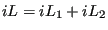 |
(133) |
This does not necessarily lead to two independent propagators, because
the two components do not commute; that is:
![$\displaystyle \exp\left[\left( iL_1 + iL_2\right)t\right] \ne \exp\left(iL_1t\right)\exp\left(iL_2t\right)$](img420.png) |
(134) |
Consider the action of the partial Liouville operator
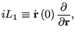 |
(135) |
which gives
The last line is the collapse of the Taylor expansion of the line
immediately above it. So, the effect of this operator fragment is a
simple shift of coordinates given some initial velocities. This is an
interesting fact: we can consider first-order integration as a Taylor
expansion.
The next step of Tuckerman was to apply the Trotter identity:
![$\displaystyle \exp\left[\left( iL_1 + iL_2\right)t\right] = \lim_{P\rightarrow\...
...\left(iL_1t/2P\right)\exp\left(iL_t2/P\right)\exp\left(iL_1t/2P\right)\right]^P$](img426.png) |
(139) |
When  is large but finite:
![$\displaystyle \exp\left[\left(iL_1 + iL_2\right)t\right] = \left[\exp\left(iL_1...
...exp\left(iL_1t/2P\right)\right]^P\exp\left[\mathscr{O}\left(1/P^2\right)\right]$](img427.png) |
(140) |
Now, we define a finite timestep as
 and we have then
a discrete operator that, when applied to a configuration at time , will
produce the configuration at time
:
and we have then
a discrete operator that, when applied to a configuration at time , will
produce the configuration at time
:
 |
(141) |
By performing this operation sequentially times, we recover a
discretized version of the formal solution to generate
 given
given
 .
.
Now we explicitly consider the decomposition:
We can perform one  's worth of update using the following operation
on :
's worth of update using the following operation
on :
The action of the rightmost operator,
 :
:
The action of the next rightmost,
 :
:
Then, the action of the final operator:
Noting that
 and
and
 , we can summarize the
effect of this three-step update of the positions and velocities as
, we can summarize the
effect of this three-step update of the positions and velocities as
This is the velocity-Verlet algorithm, seen previously in Eqs 125-127.
Interestingly, we can also reverse the order of the decomposition; i.e.,
The update algorithm that arises is
This is termed the position Verlet
algorithm [6]. Tuckerman et al. showed that
this new algorithm results in a slightly lower drift in total energy
in MD simulation of a simple Lennard-Jones fluid, when the time-step
is greater than about 0.004.
cfa22@drexel.edu
![$\displaystyle \exp\left[t\dot{\bf r}\left(0\right)\frac{\partial}{\partial{\bf r}}\right]
f\left[{\bf p}^N\left(0\right),{\bf r}^N\left(0\right)\right]$](img423.png)
![$\displaystyle \sum_{n=0}^{\infty} \frac{\left(\dot{\bf r}\left(0\right)t\right)...
...\partial{\bf r}^n}f\left[{\bf p}^N\left(0\right),{\bf r}^N\left(0\right)\right]$](img424.png)


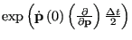
![$\displaystyle \exp\left(\dot{\bf p}\left(0\right)\left(\frac{\partial}{\partial...
...ta t}{2}\right)
f\left[{\bf p}^N\left(t\right),{\bf r}^N\left(t\right)\right]
$](img436.png)
![$\displaystyle f\left[{\bf p}^N\left(t\right),{\bf r}^N\left(t\right)\right] \ri...
... p}\left(\Delta t\right)\right]^N,\left[{\bf r}\left(t\right)\right]^N\right\}
$](img438.png)
![$\displaystyle f\left\{\left[{\bf p}\left(t\right)+\frac{\Delta t}{2}\dot{\bf p}...
...t\right)+ \Delta t \dot{\bf r}\left(\frac{\Delta t}{2}\right)\right]^N\right\}
$](img440.png)
![$\displaystyle f\left\{\left[{\bf p}\left(t\right)+\frac{\Delta t}{2}\dot{\bf p}...
...ight)+ \Delta t \dot{\bf r}\left(\frac{\Delta t}{2}\right)\right]^N\right\}\\
$](img441.png)
![$\displaystyle {\bf r}\left(0\right) +
\Delta t \dot{\bf r}\left(0\right) +
\frac{\left(\Delta t\right)^2}{2}
\frac{{\bf F}\left[{\bf r}\left(0\right)\right]}{m},$](img445.png)
![$\displaystyle \dot{\bf r}\left(0\right) + \frac{\Delta t}{2m}
\left\{{\bf F}\le...
...left(0\right)\right] + {\bf F}\left[{\bf r}\left(\Delta t\right)\right]\right\}$](img447.png)
![$\displaystyle \dot{\bf r}\left(0\right) +
\Delta t {\bf F}\left[{\bf r}\left(0\right) +
\frac{\Delta t}{2m}\dot{\bf r}\left(0\right)\right]$](img448.png)
![$\displaystyle {\bf r}\left(0\right) +
\frac{\Delta t}{2}\left[\dot{\bf x}\left(0\right)
+\dot{\bf x}\left(\Delta t\right)\right].$](img449.png)