Implementation and Evaluation

We will consider an Ewald implementation which is a modified version of the ewald code written for Berend Smit's Molecular Simulation course. (All of Prof. Smit's codes are available in the FrenkelSmitCodes directory of the instructional-codes respository.) This code simply computes the Ewald energy for a cubic lattice, given an appropriate number of particles, and a value for $\sqrt{\alpha}$ (which is called $\alpha$ in the code), and a value for $k_{\rm max}$, the maximum integer index for enumerating $k$-vectors. ¹

The units used in a system with electrostatics differ depending on community. So far, we have assumed that the units of electrostatic potential are charge $\mathscr{C}$, divided by length $\mathscr{L}$, because we write potential as $\phi = q/\vert{\bf r}\vert$, where $q$ is measured in units of $\mathscr{C}$ and distance in units of $\mathscr{L}$. Energy is therefore written in units of $\mathscr{C}^2$ over $\mathscr{L}$, and force in units of $\mathscr{C}^2$ over $\mathscr{L}^2$. If we want the final energy in more familiar units, we can choose $\mathscr{C}$ and $\mathscr{L}$, and use the standard prefactor $1/4\pi\epsilon_0$ to convert from “charge squared per length” to “energy”. For example, in SI units, $\epsilon_0 = 8.85419\times10^{-12}$ (C$^2$/m)/J. In this implementation, we use a length of $\mathscr{L} = 1$ and $\mathscr{C} = 1$ and measure energy such that $1/4\pi\epsilon_0 = 1$.

We will examine two configurations, both with $N$ = 8$^3$ = 512 particles, with alternating + and - charges. One configuration has the particle on a cubic lattice with lattice spacing $r_0 = 1$, which is the standard NaCl crystal structure. We will call this the “crystal” configuration. The other is like the crystal, only each particle is displaced by a random amount from its Self Part lattice position with a maximum displacement of 0.3. We will call this the “liquid” configuration. We compute the total electrostatic energy via the Ewald sum technique for various values of $1/\sqrt {\alpha }$ and maximum $k$-vector index. As we increase the number of $k$-vectors taken in the sum, we would like to show that the total energy converges to a certain value. We will measure this in terms of the Madelung constant, $M$:

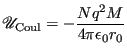$$\mathscr{U}_{\rm Coul} = -\frac{N q^2 M}{4\pi\epsilon_0r_0}$$ (257)

Table 2 shows results of Ewald summation for the perfect lattice, and Table 3 shows resuts for the “liquid”. We see several interesting things from these example calculations:

1. The self-energy is the dominant contributor from the long-range compensating charge smears.
2. The Fourier-space contribution is relatively small, and is much smaller for the perfect lattice than for the liquid. This means the precision of the Fourier transform of the charge distribution (which is larger for larger $k_{\rm max}$ is relatively unimportant to the calculation.
3. The overall Coulomb energy is insensitive to the real-space cutoff for the perfect lattice, while it is weakly decreasing in magnitude (it is negative overall) for increasing real-space cutoff in the liquid.

Table 2: Using the Ewald summation to compute total Coulomb energy of an 8x8x8 “NaCl” lattice. For various values of the real-space cutoff $1/\sqrt {\alpha }$ and maximum number of $k$-vectors $k_{\rm max}$, the values of the real-space energy $\mathscr {U}_{\rm short}$, the Fourier-space energy $\mathscr {U}_1$, and the self-energy correction $-\mathscr {U}_{\rm self}$ are shown, together with the Madelung constant $M$.

$1/\sqrt {\alpha }$	$k_{\rm max}$	$\mathscr {U}_{\rm short}$	$\mathscr {U}_1$	$\mathscr{U}_{\rm self}$	$\mathscr{U}_{\rm Coul}$	$M$
1.00	4	-0.3106	1.0354 $\times 10^{-3}$	-0.5642	-0.8738	1.7476
1.00	8	-0.3106	1.0354 $\times 10^{-3}$	-0.5642	-0.8738	1.7476
1.00	16	-0.3106	1.0354 $\times 10^{-3}$	-0.5642	-0.8738	1.7476
1.50	4	-0.4958	1.1708 $\times 10^{-7}$	-0.3780	-0.8738	1.7476
1.50	8	-0.4958	1.1708 $\times 10^{-7}$	-0.3780	-0.8738	1.7476
1.50	16	-0.4958	1.1708 $\times 10^{-7}$	-0.3780	-0.8738	1.7476
2.00	4	-0.5917	2.3491 $\times 10^{-13}$	-0.2821	-0.8738	1.7476
2.00	8	-0.5917	2.3491 $\times 10^{-13}$	-0.2821	-0.8738	1.7476
2.00	16	-0.5917	2.3491 $\times 10^{-13}$	-0.2821	-0.8738	1.7476
2.50	4	-0.6481	1.3732 $\times 10^{-20}$	-0.2257	-0.8738	1.7476
2.50	8	-0.6481	1.3732 $\times 10^{-20}$	-0.2257	-0.8738	1.7476
2.50	16	-0.6481	1.3732 $\times 10^{-20}$	-0.2257	-0.8738	1.7476
3.00	4	-0.6876	5.1260 $\times 10^{-30}$	-0.1862	-0.8738	1.7476
3.00	8	-0.6876	5.1260 $\times 10^{-30}$	-0.1862	-0.8738	1.7476
3.00	16	-0.6876	5.1260 $\times 10^{-30}$	-0.1862	-0.8738	1.7476
3.50	4	-0.7102	1.2018 $\times 10^{-36}$	-0.1636	-0.8738	1.7476
3.50	8	-0.7102	1.2018 $\times 10^{-36}$	-0.1636	-0.8738	1.7476
3.50	16	-0.7102	1.2018 $\times 10^{-36}$	-0.1636	-0.8738	1.7476
4.00	4	-0.7328	2.5866 $\times 10^{-37}$	-0.1410	-0.8738	1.7476
4.00	8	-0.7328	2.5866 $\times 10^{-37}$	-0.1410	-0.8738	1.7476
4.00	16	-0.7328	2.5866 $\times 10^{-37}$	-0.1410	-0.8738	1.7476

Table 3: Using the Ewald summation to compute total Coulomb energy of an 8x8x8 “NaCl” liquid. For various values of the real-space cutoff $1/\sqrt {\alpha }$ and maximum number of $k$-vectors $k_{\rm max}$, the values of the real-space energy $\mathscr {U}_{\rm short}$, the Fourier-space energy $\mathscr {U}_1$, and the self-energy correction $-\mathscr {U}_{\rm self}$ are shown, together with the Madelung constant $M$.

$1/\sqrt {\alpha }$	$k_{\rm max}$	$\mathscr {U}_{\rm short}$	$\mathscr {U}_1$	$-\mathscr {U}_{\rm self}$	$\mathscr{U}_{\rm Coul}$	$M$
1.00	4	-0.3322	3.1339 $\times 10^{-2}$	-0.5642	-0.8650	1.7300
1.00	8	-0.3322	3.2193 $\times 10^{-2}$	-0.5642	-0.8642	1.7283
1.00	16	-0.3322	3.2193 $\times 10^{-2}$	-0.5642	-0.8642	1.7283
1.50	4	-0.4960	9.8621 $\times 10^{-3}$	-0.3780	-0.8642	1.7283
1.50	8	-0.4960	9.8652 $\times 10^{-3}$	-0.3780	-0.8642	1.7283
1.50	16	-0.4960	9.8652 $\times 10^{-3}$	-0.3780	-0.8642	1.7283
2.00	4	-0.5859	3.8735 $\times 10^{-3}$	-0.2821	-0.8642	1.7283
2.00	8	-0.5859	3.8735 $\times 10^{-3}$	-0.2821	-0.8642	1.7283
2.00	16	-0.5859	3.8735 $\times 10^{-3}$	-0.2821	-0.8642	1.7283
2.50	4	-0.6402	1.7194 $\times 10^{-3}$	-0.2257	-0.8642	1.7283
2.50	8	-0.6402	1.7194 $\times 10^{-3}$	-0.2257	-0.8642	1.7283
2.50	16	-0.6402	1.7194 $\times 10^{-3}$	-0.2257	-0.8642	1.7283
3.00	4	-0.6787	7.4067 $\times 10^{-4}$	-0.1862	-0.8641	1.7282
3.00	8	-0.6787	7.4067 $\times 10^{-4}$	-0.1862	-0.8641	1.7282
3.00	16	-0.6787	7.4067 $\times 10^{-4}$	-0.1862	-0.8641	1.7282
3.50	4	-0.7008	3.7594 $\times 10^{-4}$	-0.1636	-0.8640	1.7281
3.50	8	-0.7008	3.7594 $\times 10^{-4}$	-0.1636	-0.8640	1.7281
3.50	16	-0.7008	3.7594 $\times 10^{-4}$	-0.1636	-0.8640	1.7281
4.00	4	-0.7230	1.5044 $\times 10^{-4}$	-0.1410	-0.8639	1.7278
4.00	8	-0.7230	1.5044 $\times 10^{-4}$	-0.1410	-0.8639	1.7278
4.00	16	-0.7230	1.5044 $\times 10^{-4}$	-0.1410	-0.8639	1.7278