Case Study: Stillinger-Weber Silicon

As a precursor to the Tersoff formalism, perhaps the earliest attempt to use molecular simulation with a reactive potential to study a realistic atomic-scale model of silicon was due to Stillinger and Weber [38]. The C-code that implements the Stillinger-Weber (SW) potential for silicon is mdswsi.c. This code computes in reduced units as well; $\sigma$ = 0.20951 nm, $\epsilon$ = 2.1678 eV, and $m$ = 28.085 amu, which are appropriate for a system of pure silicon. One reduced unit of temperature, $\epsilon/k_B$, corresponds to 25156.74 K.

The main reason to introduce Stillinger-Weber silicon here is to give you a historical example of an implementation of a simple reactive force-field. Silicon forms 4-coordinated tetrahedral bonded structures. The SW potential includes three-body interactions that enforce this symmetry as well as permit breaking and reforming of bonds to produce defects, for example.

The total potential is expressed as two sums, one for unique pair interactions, and another for unique triplet interactions:

$$\mathscr{U} = \sum_{i<j}v_2(r_{ij}) + \sum_{i<j<k}v_3({\bf r}_i, {\bf r}_j, {\bf r}_k)$$ (282)

The two-body term models the bonds:

$$v_2 \left(r\right) = \left\{\begin{array}{ll} \epsilon A \left(Br... ...\right)^{-1}\right], & \mbox{$r < a$} 0 & \mbox{$r\ge a$} \end{array} \right.$$ (283)

It is very much like a Lennard-Jones potential, only with different exponents and a “smooth cutoff” as the interatom separation distance, $r$, approaches some cutoff, $a$, given by the factor $\exp\left[\left(r-a\right)^{-1}\right]$.

The three body models the angles, and is the sum of functions of each of the three angles of a triplet, $ijk$:

$$v_3\left({\bf r}_i, {\bf r}_j, {\bf r}_k\right) = h_{jik} + h_{ijk} + h_{ikj}$$ (284)

Here I have employed the shorthand notation $$h_{jik} \equiv h\left(r_{ij}, r_{ik}, \theta_{jik}\right)$$. Note that, in the notation of this potential, $\theta _{jik}$ is subtended at ${\bf r}_i$, and $\cos\theta_{jik}^c = -\frac{1}{3}$:

$$h\left(r_{ij},r_{ik},\theta_{jik}\right) \equiv \begin{cases}\eps... ...}^c\right)^2 & \mbox{if $r_{ij} < a$, and} \cr 0 & \mbox{otherwise} \end{cases}$$ (285)

One computes the angle-$j$ term, $h_{ijk}$, and the angle-$k$ term, $h_{ikj}$, by permuting the indices appropriately.

The parameters used in the original study by Stillinger and Weber are:

$$A = 7.049556277$$ (286)

$$B = 0.6022245584$$ (287)

$$p = 4$$ (288)

$$q =$$ 0 (289)

$$a = 1.80$$ (290)

$$\lambda = 21.0$$ (291)

$$\gamma = 1.20$$ (292)

As in any MD simulation, one computes the force on any particle $i$ from the negative gradient of the total potential:

$${\bf f}_i = -\nabla_{{\bf r}_i}\mathscr{U}$$ (293)

$$= -\sum_{j\ne i} \nabla_{{\bf r}_i}v_2\left(r_{ij}\right) - \sum_{j... ...\sum_{k\ne i,j} \nabla_{{\bf r}_i}v_3\left({\bf r}_i,{\bf r}_j,{\bf r}_k\right)$$ (294)

The two-body term for the $i$-$j$ interaction is only slightly more complicated than Lennard-Jones, due to the smooth cutoff. Here, assuming $i$ and $j$ are within interaction range ( $r_{ij} < a$), we have for the force on $i$ due to $j$:

$$-\nabla_{{\bf r}_i} v_2\left(r_{ij}\right) = -\frac{\partial }{\partial{\bf r}_i} \left\{\epsilon A \left(Br_{ij}^{-p}-r_{ij}^{-q}\right)\exp\left[\left(r_{ij}-a\right)^{-1}\right]\right\}$$ (295)

$$= -\epsilon A \frac{{\bf r}_{ij}}{r_{ij}}\left(\left.\left[\frac{\p... ...)\right]\right\vert _{r_{ij}}\exp\left[\left(r_{ij}-a\right)^{-1}\right]\right.$$ (296)

$$+ \left.\left(Br_{ij}^{-p}-r_{ij}^{-q}\right)\left.\left\{\frac{\pa... ...al r}\exp\left[\left(r-a\right)^{-1}\right]\right\}\right\vert _{r_{ij}}\right)$$ (297)

$$= -\epsilon A \frac{{\bf r}_{ij}}{r_{ij}}\left\{\left(-pBr_{ij}^{-p-1}+qr_{ij}^{-q-1}\right)\exp\left[\left(r_{ij}-a\right)^{-1}\right]\right.$$ (298)

$$- \left.\left(Br_{ij}^{-p}-r_{ij}^{-q}\right)\exp\left[\left(r_{ij}-a\right)^{-1}\right]\left(r_{ij}-a\right)^{-2}\right\}$$ (299)

$$= v_2\frac{{\bf r}_{ij}}{r_{ij}}\left[\frac{pBr_{ij}^{-p-1}-qr_{ij}^{-q-1}}{Br_{ij}^{-p}-r_{ij}^{-q}} + \left(r_{ij}-a\right)^{-2}\right]$$ (300)

$$\equiv {\bf f}_{ij}$$ (301)

Note that it is still true that ${\bf f}_{ij} = -{\bf f}_{ji}$. As an exercise, you should be able to show that the right-hand-side of Eq. 300 is well-behaved (that is, it does not diverge, and in fact vanishes) as $r_{ij}\rightarrow a^-$.

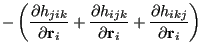
It is comparatively much more tedious to evaluate the three-body gradients:

$$-\nabla_{{\bf r}_i}v_3\left({\bf r}_i,{\bf r}_j,{\bf r}_k\right) = -\nabla_{{\bf r}_i}\left(h_{jik} + h_{ijk} + h_{ikj}\right)$$ (302)

$$= -\left(\frac{\partial h_{jik}}{\partial {\bf r}_i} +\frac{\partial h_{ijk}}{\partial {\bf r}_i} +\frac{\partial h_{ikj}}{\partial {\bf r}_i}\right)$$ (303)

$$\equiv {\bf f}_{i\leftarrow jk}$$ (304)

The triplet forces on the other members of the triplet, ${\bf f}_{j\leftarrow ik}$ and ${\bf f}_{k\leftarrow ij}$, are defined analogously.

Each of the partials in Eq. 303 is unique:

$$\begin{array}{lll} \mbox{\raisebox{-0.5cm}{\includegraphics[w... ...ik}}\frac{1}{r_{ij}}\right) \cos\theta_{jik}\right] \end{array}$$ (305)

$$\begin{array}{lll} \mbox{\raisebox{-0.5cm}{\includegraphics[w... ...j}}{r_{ij}}\frac{1}{r_{ij}} \cos\theta_{ijk}\right] \end{array}$$ (306)

$$\begin{array}{lll} \mbox{\raisebox{-0.5cm}{\includegraphics[w... ...k}}{r_{ik}}\frac{1}{r_{ik}} \cos\theta_{ikj}\right] \end{array}$$ (307)

Note that the right hand sides of each of Eqns. 305, 306, and 307 vanish when the appropriate $r$'s are greater than $a$'s, as in Eq. 212. As an exercise, it is easy to show that ${\bf f}_{i\leftarrow jk} + {\bf f}_{j\leftarrow ik} + {\bf f}_{k\leftarrow ij} = 0$.

Let us now run two MD simulations for 10,000 time steps; one with and and the other without three body forces, at reduced initial temperature $T$ = 0.12 and reduced density $\rho$ = 0.46 for a small system of 216 atoms. The code mdswsi.c can initialize atoms on a diamond-cubic lattice; the DC unit cell has 8 atoms, so the number of atoms one should specify for a perfect crystal is 8 times any product of three integers. Using the -nc #,#,# switch we indicate how may DC unit cells we want in the $x$, $y$, and $z$, directions, respectively. The code also has a switch -do-three-body which is by default on, but can be turned off by passing a zero. Running this twice generates two logs and two trajectories:

$ ./mdswsi -nc 3,3,3 -ns 10000 -fs 10 -prog 10 \ 
  -do-three-body 1 -traj yes3.xyz > yes3.log
$ ./mdswsi -nc 3,3,3 -ns 10000 -fs 10 -prog 10 \ 
  -do-three-body 0 -traj no3.xyz > no3.log

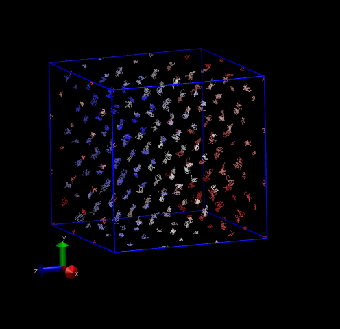
Fig. 30 shows two 3-D system representations. The first is a perfect DC lattice with 216 atoms, where a dot is drawn every 10 time steps for each atom, and each atom is colored uniquely. The second shows the same view of a system for which the three-body forces are turned off; notice that it appears liquid-like. Three-body forces are required to stabilize the DC lattice since each atom only has four nearest neighbors.

Figure 30: Two views of a 10,000-time-step NVE MD simulation of a system of 216 silicon atoms initialized on a diamond-cubic lattice; (left) with three-body force and (right) without three-body forces. Each point is an atom position, and atom positions are rendered every 10 time-steps, and each atom is colored uniquely.

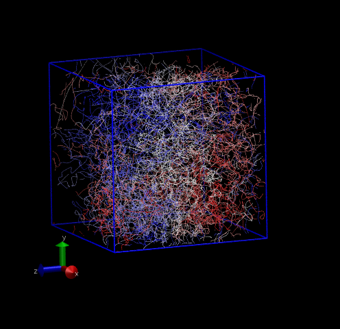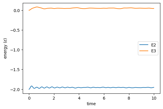
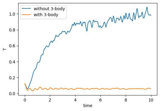
Fig. 31 shows a plot of two-body and three-body potential energy vs. time from the first simulation, and a plot of instantaneous temperature vs. time from both simulations on the right. Notice that the three-body forces act to keep the system oscillating in its crystalline state, and the lack of three-body forces results in system melting. This latter occurrence is because the DC lattice is a fairly unfavorable configuration for a system with only two-body forces active.

Figure 31: Results of a 216-atom NVE MD simulation of SW silicon initialized on a DC lattice. (Left) Two-body and three-body contributions to the potential energy vs time. (Right) Temperature vs. time for systems with and without three-body forces active.

The code mdswsi.c is very slow when three-body forces are turned on because it uses a brute-force $N^3$ loop. In practice, any code that implements two- and three-body potentials with short-range cutoffs will use data structures like the neighbor list and the link-cell algorithm to make the pair and triplet loops more efficient. And although SW silicon is historically important, there are much better (and more complicated) potentials out there for silicon-based systems, such as COMB [34].