Next: Thermodynamic Integration Up: Free Energy Methods Previous: Free Energy Methods
We recall that the free energy of the canonical ensemble, termed the
Helmholtz free energy and denoted ![]() , is defined by
, is defined by
| (308) | |||
![$\displaystyle -k_BT \ln\left(\left\{\frac{V^N}{\Lambda^{3N}N!}\right\} \left\{V...
...bf r}^N \exp\left[-\beta\mathscr{U}\left({\bf r}^N\right)\right]\right\}\right)$](img819.png) |
(309) | ||
![$\displaystyle -k_BT\ln\left(\frac{V^N}{\Lambda^{3N}N!}\right) - k_BT\ln\left(\int d{\bf s}^N \exp\left[-\beta\mathscr{U}\left({\bf s}^N;L\right)\right]\right)$](img820.png) |
(310) | ||
| (311) |
Here,
![]() is the “ideal gas” free energy, and
is the “ideal gas” free energy, and
![]() is the “excess” free energy. The chemical potential is defined as the change in free energy upon
addition of a particle:
is the “excess” free energy. The chemical potential is defined as the change in free energy upon
addition of a particle:
 |
(312) |
For large ![]() ,
,
| (313) | |||
![$\displaystyle -k_BT\ln\left(\frac{V/\Lambda^d}{N+1}\right) - k_BT\ln\left(
\fra...
...cr{U}\left({\bf s}^{N};L\right)\right]
\end{displaymath}\end{minipage}}}\right)$](img827.png) |
(314) | ||
| (315) |
 |
(316) |
The code mclj_widom.c
implements the Widom method for the Lennard-Jones fluid in an NVT
simulation. Below is a code fragment for sampling
![]() using the Lennard-Jones pair potential 89:
using the Lennard-Jones pair potential 89:
  rx[N]=(gsl_rng_uniform(r)-0.5)*L;
  ry[N]=(gsl_rng_uniform(r)-0.5)*L;
  rz[N]=(gsl_rng_uniform(r)-0.5)*L;

  for (j=0;j<N;j++) {
    dx  = rx[N]-rx[j];
    dy  = ry[N]-ry[j];
    dz  = rz[N]-rz[j];
    r2  = dx*dx + dy*dy + dz*dz;
    r6i = 1.0/(r2*r2*r2);
    du += 4*(r6i*r6i - r6i);
  }
The particle with index ![]() is assumed to be the “test particle”;
the other particles are indexed 0 to
is assumed to be the “test particle”;
the other particles are indexed 0 to ![]() . In the first bit, the
position of the test particle is generated as a uniformly random
location inside a cubic box of side length
. In the first bit, the
position of the test particle is generated as a uniformly random
location inside a cubic box of side length ![]() . Then we loop over the
particles 0 to
. Then we loop over the
particles 0 to ![]() and accumulate
and accumulate
![]() .
.
Using the code mclj_widom.c, we can measure
![]() in NVT MC simulations. This represents an alternate way of computing
in NVT MC simulations. This represents an alternate way of computing
![]() to that of
to that of ![]() MC, in which
MC, in which ![]() is an observable.
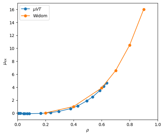
In Fig. 39, I show
is an observable.
In Fig. 39, I show
![]() vs.
vs. ![]() at
at ![]() = 3.0 computed using both
= 3.0 computed using both ![]() MC and the NVT Widom method. The
MC and the NVT Widom method. The ![]() simulations were initialized with 512 particles initially, while the Widom simulations were run with
simulations were initialized with 512 particles initially, while the Widom simulations were run with ![]() = 216 particles. Each point is an average of three indenpemdent calculations.
= 216 particles. Each point is an average of three indenpemdent calculations.
 |
It would be useful to know how to determine which of these apparently
competing methods is best for computing
![]() . They are both
similar in computational requirements (this is not further qualified
here; if someone wants to make this comparison, he or she is welcome
to do this as a project). On the one hand, we have an inherent
limitation of the grand canonical simulation: one cannot specify the
system density exactly; rather it is an observable with some mean and
fluctuations. The Widom method does allow one to specify the density
precisely, and in this regard, it is probably more trustworthy in
computing
. They are both
similar in computational requirements (this is not further qualified
here; if someone wants to make this comparison, he or she is welcome
to do this as a project). On the one hand, we have an inherent
limitation of the grand canonical simulation: one cannot specify the
system density exactly; rather it is an observable with some mean and
fluctuations. The Widom method does allow one to specify the density
precisely, and in this regard, it is probably more trustworthy in
computing
![]() . On the other hand, the Widom method suffers
the limitation that it is not generally applicable to systems with any
potential energy function. For example, for hard-sphere systems, the
Widom method would always predict that
. On the other hand, the Widom method suffers
the limitation that it is not generally applicable to systems with any
potential energy function. For example, for hard-sphere systems, the
Widom method would always predict that
![]() is 0, a clearly
nonsensical answer. The “overlapping distribution method” of
Bennett, discussed in Section 7.2.3 of F&S, offers a means to overcome
this particular limitation. We do not cover this method in lecture,
but you are encouraged to explore the overlapping distribution method
on your own (maybe as a project).
is 0, a clearly
nonsensical answer. The “overlapping distribution method” of
Bennett, discussed in Section 7.2.3 of F&S, offers a means to overcome
this particular limitation. We do not cover this method in lecture,
but you are encouraged to explore the overlapping distribution method
on your own (maybe as a project).
cfa22@drexel.edu