Next: Case Study 3: Transport Up: Case Study 2: Static Previous: Equilibration and Decorrelation
A second major objective of this case study is to demonstrate how to
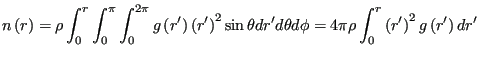
compute the radial distribution function, ![]() . The radial
distribution function is an important statistical mechanical function
that captures the structure of liquids and amorphous solids. We can
express
. The radial
distribution function is an important statistical mechanical function
that captures the structure of liquids and amorphous solids. We can
express ![]() using the following statement:
using the following statement:
 |
(157) |
The procedure we will follow will be to write a second program (a
“postprocessing code”) which will read in the trajectory output
produced by the simulation, mdlj.c.
The general structure of a ![]() post-processing code could look
like this:
post-processing code could look
like this:
We will consider a code, rdf.c, that
implements this algorithm for computing ![]() , but first we present a
brief argument for post-processing vs on-the-fly processing for
computing quantities such as
, but first we present a
brief argument for post-processing vs on-the-fly processing for
computing quantities such as ![]() . For demonstration purposes, it
is arguably simpler to drop in a
. For demonstration purposes, it
is arguably simpler to drop in a ![]() -histogram update sampling
function into an existing MD simulation program to enable computation
of
-histogram update sampling
function into an existing MD simulation program to enable computation
of ![]() during a simulation, compared to writing a wholly
separate program. After all, it nominally involves less coding. The
counterargument is that, once you have a working (and eventually
optimized) MD simulation code, one should be wary of modifying it.
The purpose of the MD simulation is to produce samples. One can
produce samples once, and use any number of post-processing codes to
extract useful information. The counterargument becomes stronger when
one considers that, for particularly large-scale simulations, it is
simply not convenient to re-run an entire simulation when one
discovers a slight bug in the sampling routines. The price one
pays is that one needs the disk space to store configurations.
during a simulation, compared to writing a wholly
separate program. After all, it nominally involves less coding. The
counterargument is that, once you have a working (and eventually
optimized) MD simulation code, one should be wary of modifying it.
The purpose of the MD simulation is to produce samples. One can
produce samples once, and use any number of post-processing codes to
extract useful information. The counterargument becomes stronger when
one considers that, for particularly large-scale simulations, it is
simply not convenient to re-run an entire simulation when one
discovers a slight bug in the sampling routines. The price one
pays is that one needs the disk space to store configurations.
As shown earlier, one MD simulation of 108 particles out to 600,000
time steps, storing configurations every 1,000 time steps, requires
less than 5 MB. This is an insignificant price. Given that we know that the MD simulation works correctly, it is sensible to leave it alone and write a quick, simple post-processing code to read
in these samples and compute ![]() .
.
The code rdf.c is a C-code implementation
of just such a post-processing code. This program illustrates a different way to abstractify the trajectory, namely as a list of frames. A frame is an instance of an abstract data type called frametype that we define (for now) in rdf.c, along with a special function NewFrame() to allocate memory for a frame, and another read_xyz_frame() to read a frame in from an XYZ-format trajectory:
typedef struct FRAME {
    double * rx, * ry, * rz;  // coordinates
    double * vx, * vy, * vz;  // velocities
    int * typ; // array of particle types 0, 1, ...
    int N; // number of particles
    double Lx, Ly, Lz; // box dimensions
} frametype;

/* Create and return an empty frame */
frametype * NewFrame ( int N, int hv ) {
    frametype * f = (frametype*)malloc(sizeof(frametype));
    f->N=N;
    f->rx=(double*)malloc(sizeof(double)*N);
    f->ry=(double*)malloc(sizeof(double)*N);
    f->rz=(double*)malloc(sizeof(double)*N);
    if (hv) {
        // caller has requested a frame with space for velocities
        f->vx=(double*)malloc(sizeof(double)*N);
        f->vy=(double*)malloc(sizeof(double)*N);
        f->vz=(double*)malloc(sizeof(double)*N);
    } else {
        f->vz=NULL;
        f->vy=NULL;
        f->vx=NULL;
    }
    f->typ=(int*)malloc(sizeof(int)*N);
    return f;
}
/* Read an XYZ-format frame from stream fp; returns the new frame.
   Note the non-conventional use of the first line to indicate
   whether or not the frame contains velocities and the comment
   line to hold boxsize information. */
frametype * read_xyz_frame ( FILE * fp ) {
    int N,i,j,hasvel=0;
    double x, y, z, Lx, Ly, Lz, vx, vy, vz;
    char typ[3], dummy[5];
    char ln[255];
    frametype * f = NULL;
    if (fgets(ln,255,fp)){
        sscanf(ln,"%i %i\n",&N,&hasvel);
        f = NewFrame(N,hasvel);
        fgets(ln,255,fp);
        sscanf(ln,"%s %lf %lf %lf\n",dummy,&f->Lx,&f->Ly,&f->Lz);
        for (i=0;i<N;i++) {
            fgets(ln,255,fp);
            sscanf(ln,"%s %lf %lf %lf %lf %lf %lf\n",
                   typ,&f->rx[i],&f->ry[i],&f->rz[i],&vx,&vy,&vz);
            if (hasvel) {
                f->vx[i]=vx;
                f->vy[i]=vy;
                f->vz[i]=vz;
            }
            j=0;
            while(strcmp(elem[j],"NULL")&&strcmp(elem[j],typ)) j++;
            if (strcmp(elem[j],"NULL")) f->typ[i]=j;
            else f->typ[i]=-1;
        }
    }
    return f;
}
With this abstract data type, we no longer need to pass all parallel arrays as separate parameters; we can instead just pass a pointer frametype*. For example, below is the function rij that computes the minimum-image convention distance between particles i and j in a particular frame:
/* Compute scalar distance between particles i and j in frame f;
   note the use of the minimum image convention */
double rij ( frametype * f, int i, int j ) {
    double dx, dy, dz;
    double hLx=0.5*f->Lx,hLy=0.5*f->Ly,hLz=0.5*f->Lz;
    dx=f->rx[i]-f->rx[j];
    dy=f->ry[i]-f->ry[j];
    dz=f->rz[i]-f->rz[j];
    if (dx<-hLx) dx+=f->Lx;
    if (dx> hLx) dx-=f->Lx;
    if (dy<-hLy) dy+=f->Ly;
    if (dy> hLy) dy-=f->Ly;
    if (dz<-hLz) dz+=f->Lz;
    if (dz> hLz) dz-=f->Lz;
    return sqrt(dx*dx+dy*dy+dz*dz);
}
Using rij() it is then easy to update the RDF histogram:
/* An N^2 algorithm for computing interparticle separations
   and updating the radial distribution function histogram. */
void update_hist ( frametype * f, double rcut,
                   double dr, int * H, int nbins ) {
    int i,j;
    double r;
    int bin;
    for (i=0;i<f->N-1;i++) {
        for (j=i+1;j<f->N;j++) {
            r=rij(f,i,j);
            if (r<rcut) {
                bin=(int)(r/dr);
                if (bin<0||bin>=nbins) {
                    fprintf(stderr,
                            "Warning: %.3lf not on [0.0,%.3lf]\n",
                            r,rcut);
                } else {
                    H[bin]+=2;
                }
            }
        }
    }
}
H is the histogram. One can see that the bin value is computed by first dividing the actual distance between members of
the pair by the resolution of the histogram, ![]() , and casting the result as an integer. This
resolution can be specified on the command-line when
, and casting the result as an integer. This
resolution can be specified on the command-line when rdf.c is
executed. Also notice that the histogram is updated by 2, which
reflects the fact that either of the two particles in the pair can be
placed at the origin. Also notice the implementation of the
minimum image convention.
In the main() function of rdf.c, a simple block of code can read in a whole
trajectory from a file named by trajfile and store it in an array of frametype* pointers:
    i=0;
    fprintf(stdout,"Reading %s\n",trajfile);
    fp=fopen(trajfile,"r");
    while (Traj[i++]=read_xyz_frame(fp));
    nFrames=i-1;
    fclose(fp);
    if (!nFrames) {
        fprintf(stdout,"Error: %s has no data.\n",trajfile);
        exit(-1);
    }
    fprintf(stdout,"Read %i frames from %s.\n",nFrames,trajfile);
Then a second block of code allocates, initializes, and computes the pair correlation histogram:
    /* Adjust cutoff and compute histogram */
    L2min=min(Traj[0]->Lx/2,min(Traj[0]->Ly/2,Traj[0]->Lz/2));
    if (rcut>L2min) rcut=L2min;
    nbins=(int)(rcut/dr)+1;
    H=(int*)malloc(sizeof(int)*nbins);
    for (i=0;i<nbins;i++) H[i]=0;
    for (i=begin_frame;i<nFrames;i++)
        update_hist(Traj[i],rcut,dr,H,nbins);
    nFramesAnalyzed=nFrames-begin_frame;
Note that the cutoff rcut may not exceed half a box length in any dimension. The number of histogram bins is simply one plus the cutoff divided by the resolution dr. The variable begin_frame allows the caller to gather statistics only after a certain number of frames in the trajectory in order to “ignore” initial frames where the initial configuration is still “remembered”.
Finally, once the trajectory has been traversed and the histrogram computed, it is then normalized by compute ![]() and save the result to a designated output file:
and save the result to a designated output file:
    /* Normalize and output g(r) to the terminal */
    /* Compute density, assuming NVT ensemble */
    fp=fopen(outfile,"w");
    fprintf(fp,"# RDF from %s\n",trajfile);
    fprintf(fp,"#LABEL r g(r)\n");
    fprintf(fp,"#UNITS %s *\n",length_units);
    /* Ideal-gas global density; assumes V is constant */
    rho=Traj[0]->N/(Traj[0]->Lx*Traj[0]->Ly*Traj[0]->Lz);
    for (i=0;i<nbins-1;i++) {
        /* bin volume */
        vb=4./3.*M_PI*((i+1)*(i+1)*(i+1)-i*i*i)*dr*dr*dr;
        /* number of particles in this shell if this were
           an ideal gas */
        nid=vb*rho;
        fprintf(fp,"%.5lf %.5lf\n",i*dr,
                (double)(H[i])/(nFramesAnalyzed*Traj[0]->N*nid));
    }
    fclose(fp);
    fprintf(stdout,"%s created.\n",outfile);
(The variable length_units is a string that just labels the length units; by default, this
is "sigma", indicating LJ
Now, let's execute rdf from one of our 600,000-time-step simulations' 6,001-frame trajectory, ignoring the first 1,000 frames (100,000 time steps):
$ cd ~/dxu/chet580/instructional-codes/my_work/mdlj/set1
$ gcc -O5 -o rdf ../../../originals/rdf.c -lm
$ ./rdf -t traj-rho0.90-rep0.xyz -dr 0.02 -rcut 3.5 \
   -o rdf-rho0.90-rep0.dat -begin-frame 1000
Reading traj-rho0.90-rep0.xyz
Read 6001 frames from traj-rho0.90-rep0.xyz.
rdf-rho0.90-rep0.dat created.
$
Using the python program plot_rdf.py, we can generate a plot of this RDF (Fig. 17:
$ python ../../../originals/plot_rdf.py -i rdf-rho0.90-rep0.dat \
  -o rdf-rho0.90-rep0.png
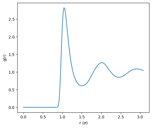 |
This ![]() shows a peak at about 2
shows a peak at about 2
![]() that corresponds to the LJ well, indicating that there is a dense nearest-neighbor shell out to about 1.5
that corresponds to the LJ well, indicating that there is a dense nearest-neighbor shell out to about 1.5 ![]() . How dense? We can use
. How dense? We can use ![]() to count particles within a distance
to count particles within a distance ![]() from a
central atom:
from a
central atom:
plot_rdf.py via the -rho and -R flags:
$ python ../../../originals/plot_rdf.py -i rdf-rho0.90-rep0.dat \
  -o rdf-rho0.90-rep0.png -rho 0.9 -R 1.5
n=12.335
This indicates the nearest neighbor shell is pretty well packed; spherical close-packing would be exactly 12.
cfa22@drexel.edu