Equilibration and Decorrelation

An important purpose of this case study is to quantify the notion of “equilibration” of the system by assessing correlations in (apparently) randomly fluctuating quantities like potential energy. Remember, in order to perform accurate ensemble averaging over an MD trajectory, we have to be sure that correlations in the properties we are measuring have “died out.” This is another way of saying that the length of the time interval over which we conduct the time average must be much longer than the correlation time. In this case study, we illustrate the “block averaging” technique of Flyvbjerg and Petersen [7] to determine the equilibration time-scale of the potential energy.

First, compute the variance of the $L$ samples of $\mathscr{U}$:

$$\sigma^2_0\left({\mathscr{U}}\right) \approx \frac{1}{L}\sum_{i=1}^{L}\left[\mathscr{U}_i - \bar{\mathscr{U}}\right]^2$$ (155)

This is approximate because of so far undetermined time-correlations in $\mathscr{U}$; that is, not all $L$ samples are uncorrelated. For example, two samples one time-step apart will likely be very close to one another. Now, we block the data by averaging $L/2$ pairs of adjacent values:

$$\mathscr{U}_i^{(1)} = \frac{\mathscr{U}_{2i-1} + \mathscr{U}_{2i}}{2}$$ (156)

The $(1)$ superscript indicates that this is a “first-generation” coarsening of the potential energy trace. The variance of this new set, $\sigma^2_1$ is computed. Then the process is recursively carried out through many subsequent generations. After many blocking operations, the coarsened samples, $\mathscr{U}_i^{(j)}$, become uncorrelated, and the variance saturates (temporarily). This means we should observe a plateau in a plot of variance vs generation. The Python program flyvberg.py implements this calculation using outputs of mdlj.c as inputs.

Figure 16: The standard deviation, $\sigma$, of potential energy per particle vs. number of blocking operations $M$ for a simulations of 150,000 and 600,000 time-steps: initial temperature $T_0$ = 0.729, density $\rho$ = 0.8442, number of particles $N$ = 108.

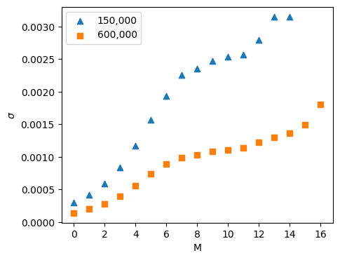According to the discussion of this blocking technique, the standard deviation shows a dependence on the blocking degree, $M$, when the blocked averages are correlated, and plateaus at a blocking degree for which the averages become uncorrelated. This blocking degree corresponds to a time interval of length $2^M$. This data indicates that potential energy decorrelates after a time of approximately $2^{10} \approx 1000$ steps. This is a reassuring result, as we could have guessed that 1000 steps are required based on the initial transience in the energy traces seen in the previous figure. I ran three independent simulations, each differing only in the random number seed used. The results are shown in Table 1.

Table 1: Average potential energy per particle $\mathscr {U}/N$, kinetic energy $\mathscr {K}/N$, total energy $\mathscr {T}$/N, and pressure $P$ (all in Lennard-Jones units) for three distinct $N$=108 particle systems run for 600,000 time steps at number density $\rho$ = 0.8442 and initial temperature $T_0$ of 0.728.

Run	$\left<\mathscr{U}\right>/N$	$\left<\mathscr{K}\right>/N$	$\left<\mathscr{T}\right>$	$\left<P\right>$
1	$-4.4165 \pm 0.0012$	$2.2577 \pm 0.0012$	$1.5051 \pm 0.0008$	$5.1960 \pm 0.0057$
2	$-4.4188 \pm 0.0010$	$2.2597 \pm 0.0010$	$1.5064 \pm 0.0007$	$5.1948 \pm 0.0050$
3	$-4.4157 \pm 0.0011$	$2.2564 \pm 0.0011$	$1.5043 \pm 0.0008$	$5.2022 \pm 0.0055$
Avg.	$-4.4170 \pm 0.0011$	$2.2579 \pm 0.0011$	$1.5053 \pm 0.0008$	$5.1977 \pm 0.0054$