Velocity Rescaling: Isokinetics and the Berendsen Thermostat

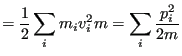
“Isokinetics” refers to altering velocities on the fly to keep kinetic energy (and therefore temperature) constant. The relationship between kinetic energy and temperature results from the application of the equipartition theorem to velocity (or, equivalently, momentum) degrees of freedom:

$$\frac{3}{2}Nk_BT = \frac{1}{2}\sum_im_iv_i^2m = \sum_i\frac{p_i^2}{2m}$$ (201)

Scaling every particle velocity by a factor $\lambda$ will yield a new temperature $T^\prime$:

$$\lambda = \sqrt{\left(T^\prime/T\right)}$$ (202)

An isokinetic thermostat computes $\lambda$ and rescales velocities at every time step. Such a thermostat cannot be used to conduct a simulation in the canonical ensemble, since it totally suppresses the required temperature fluctuations. However, isokinetics is perfectly fine to use in a warmup or initialization phase in order to prevent numerical instabilities.

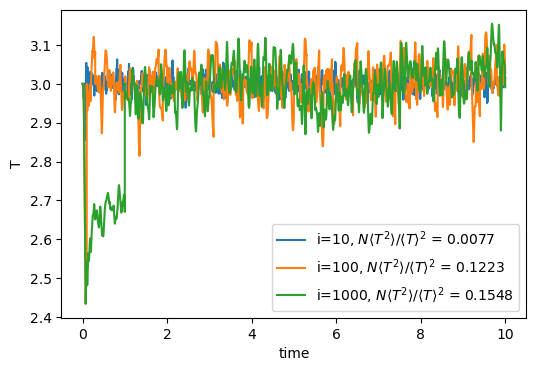
The code mdlj_isok.c illustrates implementation of an isokinetic thermostat for constant-$T$ simulation of a Lennard-Jones fluid. The implementation uses a two parameters, isoKT and isoKi, that specify the desired temperature and the number of time steps between applications of the rescaling. It is worth asking whether or not occasional velocity rescaling (rather than at every step) might allow us to preserve the correct statistics. Fig. 22 shows traces of temperature vs time for three MD simulations of the Lennard-Jones fluid with 512 particles at a density of 0.50. Each simulation used a different interval size i. The quantity $N\frac{\langle T^2\rangle - \langle T\rangle^2}{\langle T\rangle^2}$ is computed for each set and values are shown in the legend. For pure canonical statistics, we know this should be 2/3; clearly, isokinetics even at a very modest frequency utterly fails to preserve canonical statistics.

Figure 22: Temperature vs time (output every time step) for three isokinetic MD simulations of the LJ fluid at density 0.5 with 512 particles. $i$ indicates the number of steps between velocity rescalings; the setpoint temperature is 3.0, and all simulations were initialized with velocities consistent with a temperature of 2.0.

Berendsen realized that velocity scaling could be reformulated to model energy exchange with a bath at constant $T$ [9]. His scale factor is defined as

$$\lambda = \left[1+\frac{\Delta t}{\tau_T}\left(\frac{T_0}{T} - 1\right)\right]^{\frac{1}{2}}$$ (203)

Here, $T_0$ is the setpoint temperature, $\Delta t$ is the integration time step, and $\tau_T$ is a constant called the “rise time” of the thermostat. It describes the strength of the coupling of the system to a hypothetical heat bath. The larger $\tau_T$, the weaker the coupling; in other words, the larger $\tau_T$, the longer it takes to achieve a given $T_0$ after an instantaneous change from some previous $T_0$.

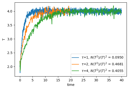
The code mdlj_ber.c implements the Berendsen thermostat. The two relevant parameters are berT, the setpoint temperature, and ber_tau, the rise time. Fig. 23 shows traces of temperature vs time for three MD simulations of the Lennard-Jones fluid with 512 particles at a density of 0.50, with temperature controlled using the Berendsen thermostat with various values of $\tau$. Larger $\tau$ clearly results in longer approach times to the setpoint temperature. Note also that the relative fluctuations of the temperature reported indicate that canonical statistics are not being held.

Figure 23: Temperature vs time (output every time step) for three Berendsen-thermostatted MD simulations of the LJ fluid at density 0.5 with 512 particles. $\tau$ indicates the rise time; the setpoint temperature is 3.0, and all simulations were initialized with velocities consistent with a temperature of 2.0.

Though relatively simple, velocity scaling thermostats are not recommended for use in production MD runs because they do not strictly conform to the canonical ensemble.