Stochastic NVT Thermostats: Andersen, Langevin, and Dissipative Particle Dynamics

The Andersen Scheme. Perhaps the simplest thermostat which does correctly sample the NVT ensemble is due to Andersen [10]. Here, at each step, some prescribed number of particles is selected, and their momenta (actually, their velocities) are drawn from a Gaussian distribution at the prescribed temperature (otherwise known as the Maxwell-Boltzmann distribution):

$$\mathscr{P}(p) = \left(\frac{\beta}{2\pi m}\right)^{3/2} \exp\left[-\beta p^2/\left(2m\right)\right]$$ (204)

This is intended to mimic collisions with bath particles at a specified $T$. The strength of the coupling to the heat bath is specified by a collision frequency, $\nu$. For each particle, a random variate is selected between 0 and 1. If this variate is less than $\nu\Delta t$, then that particle's momenta are reset.

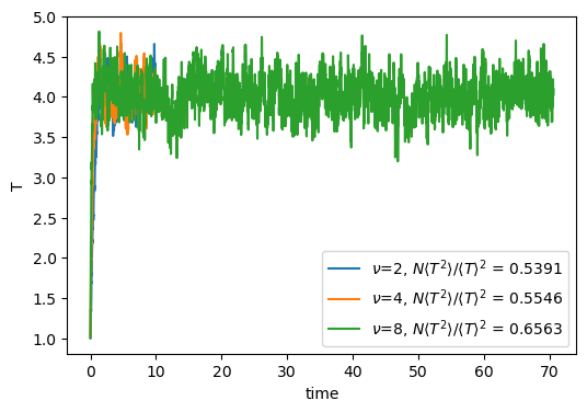
The code mdlj_and.c implements the Andersen thermostat for the Lennard-Jones fluid. The two relevant parameters are and_T, the setpoint temperature, and and_nu, the rise time. Fig. 24 shows traces of temperature vs time for three MD simulations of the Lennard-Jones fluid with 512 particles at a density of 0.50, with temperature controlled using the Andersen thermostat with various values of collision frequency $\nu$. Larger $\nu$ results in longer approach times to the setpoint temperature, but it is also clear that for these values of $\nu$, the Andersen thermostat acts much more quickly than the Berendsen thermostat. Note also that the relative fluctuations of the temperature reported indicate that canonical statistics are in fact being held.

Figure 24: Temperature vs time (output every time step) for three Berendsen-thermostatted MD simulations of the LJ fluid at density 0.5 with 512 particles. $\tau$ indicates the rise time; the setpoint temperature is 3.0, and all simulations were initialized with velocities consistent with a temperature of 2.0.

Although temperature fluctuations match the canonical ensemble, the Andersen thermostat destroys momentum transport because of the random reassignment of velocities; hence, there is no continuity of momentum in an Andersen LJ fluid, and therefore no proper $\mathscr{D}$ or viscosity. Fig. 6.3 in Frenkel & Smit clearly shows that $\mathscr{D}$, if measured from an Andersen MD run, is incorrect.

The Langevin thermostat. In the “Langevin” thermostat, at each time step all particles receive a random force and have their velocities lowered using a constant friction. [11] The average magnitude of the random forces and the friction are related in a particular way, which guarantees that the “fluctuation-dissipation” theorem is obeyed, thereby guaranteeing NVT statistics.

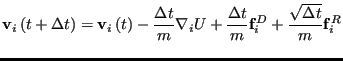
In this formalism, the particle-$i$ equation of motion is modified:

$$m\ddot{\bf r}_i = -\nabla_i U - m\Gamma\dot{\bf r}_i + {\bf W}_i\left(t\right)$$ (205)

Here, $\Gamma$ is a friction coefficient with units of $\tau^{-1}$, and ${\bf W}_i$ is a random force that is uncorrelated in time and across particles, with a mean given by

$$\left<{\bf W}_i\left(t\right),{\bf W}_j\left(t^\prime\right)\right> = \delta_{ij}\delta\left(t-t^\prime\right)6k_BmT\Gamma$$ (206)

The code mdlj_lan.c implements the Langevin thermostat. The two relevant parameters are lanT, the setpoint temperature, and lan_friction, the friction $\Gamma$. The two major elements are a force initialization at each time step that adds in the random forces, ${\bf W}$, and a slight modification to the update equations in the integrator to include the effect of $\Gamma$. Note that the initialization of forces to zero in the force routine has been removed.

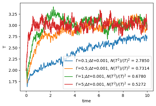
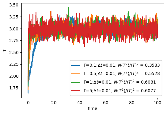
Fig. 25 shows temperature vs time for several MD simulations of a 512-particle LJ fluid at a density of 0.5; the upper plot shows data from runs with $\Delta t$=10$^{-3}$, and the lower plot $\Delta t$=10$^{-2}$, each showing four values of $\Gamma$. Relative temperature fluctuations indicate weak agreement with canonical statistics that improves for the lower values of $\Delta t$.

Figure 25: Temperature vs time (output every time step) for eight Langevin-thermostatted MD simulations of the LJ fluid at density 0.5 with 512 particles. $\Gamma$ indicates the friction; the setpoint temperature is 3.0, and all simulations were initialized with velocities consistent with a temperature of 2.0. Upper plot shows $\Delta t$ of 0.001, lower 0.01.

One advantage of the Langevin thermostat (and to a limited extent, the Andersen thermostat and other stochastic-based thermostats) is that we can get away with a larger time step than in NVE simulations. At a density of $\rho$ = 0.8442 and a mean temperature $T$ = 1.0, an NVE simulation is unstable for time-steps above about $\Delta t$ = 0.004. We can, however, run a Langevin dynamics simulation with a friction $\Gamma$ = 1.0 stably with a time-step as large as $\Delta t$ = 0.01 or even higher. This has proven invaluable in simulations of more complicated systems that simple liquids, namely linear polymers, which have very long relaxation times. MD with the Langevin thermostat is the method of choice for equilibrating samples of liquids of long bead-spring polymer chains.

Of course, the drawback of most stochastic thermostats (one exception is discussed next) is that momentum transfer is destroyed. So again, it is unadvisable to use Langeving or Andersen thermostats for runs in which you wish to compute diffusion coefficients. The recommendation stands: use NVE to compute properties, and use thermostats for equilibration only.

The Dissipative Particle Dynamics thermostat. The DPD thermostat [12,13] adds pairwise random and dissipative forces to all particles, and has been shown to preserve momentum transport. Hence, it is the only stochastic thermostat so far that should even be considered for use if one wishes to compute transport properties.

The DPD thermostat is implemented by slight modification of the force routine to add in the pairwise random and dissipative forces. For the $ij$ pair, the dissipative force is defined as

$${\bf f}_{ij}^D = -\gamma\omega^D\left(r_{ij}\right)\left({\bf v}_{ij}\cdot\hat{\bf r}_{ij}\right)\hat{\bf r}_{ij}$$ (207)

Here, $\gamma$ is a friction coefficient, $\omega$ is a cut-off function for the force as a function of the scalar distance between $i$ and $j$ which simply limits the interaction range of the dissipative (and random) forces, ${\bf v}_{ij} = {\bf v}_i - {\bf v}_j$ is the relative velocity of $i$ to $j$, and $\hat{\bf r}_{ij} = {\bf r}_{ij}/r_{ij}$ is the unit vector pointing from $j$ to $i$. The random force is defined as

$${\bf f}_{ij}^R = \sigma\omega^R\left(r_{ij}\right)\zeta_{ij}\hat{\bf r}_{ij}$$ (208)

Here, $\sigma$ is the strength of the random force, $\omega^R$ is a cut-off, and $\zeta_{ij}$ is a Gaussian random number with zero mean and unit variance, and $\zeta_{ij} = \zeta_{ji}$.

The update of velocity uses these new forces:

$${\bf v}_i\left(t + \Delta t\right) = {\bf v}_i\left(t\right) - \f... ...nabla_iU + \frac{\Delta t}{m}{\bf f}_i^D + \frac{\sqrt{\Delta t}}{m}{\bf f}_i^R$$ (209)

where

$${\bf f}_i^D = \sum_{j\ne i} {\bf f}_{ij}^D$$ (210)

$${\bf f}_i^R = \sum_{j\ne i} {\bf f}_{ij}^R$$ (211)

The parameters $\gamma$ and $\sigma$ are linked by a fluctuation-dissipation theorem:

$$\sigma^2 = 2\gamma k_B T$$ (212)

So, in practice, one must specify either $\gamma$ or $\sigma$, and then a setpoint temperature, $T$, in order to use the DPD thermostat.

The cutoff functions are also related:

$$\omega^D\left(r_{ij}\right) = \left[\omega^R\left(r_{ij}\right)\right]^2$$ (213)

This is the only real constraint on the cutoffs; we are otherwise allowed to use any cutoff we like. The simplest uses the cutoff radius of the pair potential, $r_c$:

$$\omega\left(r\right) = \left\{\begin{tabular}{ll} 1 & \mbox{$r < r_c$} 0 & \mbox{$r > r_c$} \end{tabular}\right.$$ (214)

Note that, with this choice, $\left[\omega^R\left(r_{ij}\right)\right]^2$ = $\omega^R\left(r_{ij}\right)$ = $\omega^D\left(r_{ij}\right) = \omega$.

The code mdlj_dpd.c implements the DPD thermostat in an MD simulation of the Lennard-Jones liquid. The major changes (compared to mdlj.c) are to the force routine, which now requires several more arguments, including particle velocities, and parameters for the thermostat. Inside the pair loop, the force on each particle is updated by the conservative, dissipative, and random pairwise force components. The random force is divided by $\sqrt{\Delta t}$ so that the velocity Verlet algorithm need not be altered to implement Eq. 209.

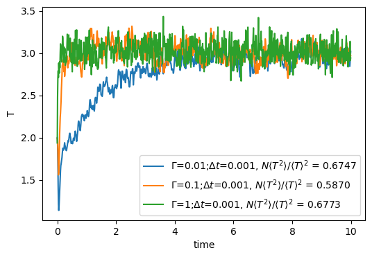
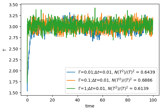
The behavior of the DPD thermostat can be assessed in a similar fashion as was the Berendsen thermostat above. Here I've run several MD simulations of the LJ fluid at a density of 0.84 with 512 particles for 10,000 steps, with various values of $\Gamma$ and $\Delta t$. Fig. 26 shows the temperature vs time for these various runs. We see that increased friction leads to faster approach to the setpoint temperature, and that temperature fluctuations seem to conform to canonical statistics pretty well.

Figure 26: Temperature vs time (output every time step) for eight DPD-thermostatted MD simulations of the LJ fluid at density 0.84 with 512 particles. $\Gamma$ indicates the friction; the setpoint temperature is 3.0, and all simulations were initialized with velocities consistent with a temperature of 2.0. Upper plot shows $\Delta t$ of 0.001, lower 0.01.