Next: Ewald Forces Up: Long-Range Interactions: The Ewald Previous: Long-Range Interactions: The Ewald
First, assume we have a collection of charged particles in a cubic box
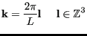
with side length ![]() , with periodic boundary conditions. The
collection is assumed neutral; there is an equal number of positive
and negative charges. The total Coulombic energy in this system is
given by:
, with periodic boundary conditions. The
collection is assumed neutral; there is an equal number of positive
and negative charges. The total Coulombic energy in this system is
given by:
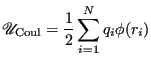 |
(226) |
![]() is the electrostatic potential at position
is the electrostatic potential at position ![]() :
:
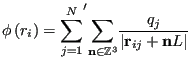 |
(227) |
To evaluate
![]() efficiently, we break it into two parts:
efficiently, we break it into two parts:
How can we do this? The idea of Ewald is to do two things: first,
screen each point charge using a diffuse cloud of opposite charge
around each point charge, and then compensate for these screening
charges using a smoothly varying, periodic charge density. The
screening charge is constructed to make the electrostatic potential
due to a charge at position ![]() decay rapidly to near zero at a
prescribed distance. These interactions are treated in real space.
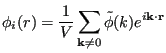
The compensating charge density, which is the sum of all screening
densities except with opposite charges, is treated using a Fourier
series.
decay rapidly to near zero at a
prescribed distance. These interactions are treated in real space.
The compensating charge density, which is the sum of all screening
densities except with opposite charges, is treated using a Fourier
series.
The standard choice for a screening potential is Gaussian:
| (228) |
So for each charge, we add such a screening potential. Now, to
evaluate
![]() , we have to evaluate the potential
of a charge density that compensates for the screening charge
densities at each particle. This is done in Fourier space.
, we have to evaluate the potential
of a charge density that compensates for the screening charge
densities at each particle. This is done in Fourier space.
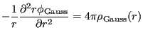
The potential of a given charge distribution is given by Poisson's equation:
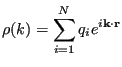
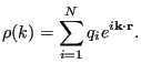
Now, the compensating charge distribution, denoted ![]() , can be
written:
, can be
written:
![$\displaystyle \rho_1(r) = \sum_{j=1}^{N}\sum_{{\bf n}\in\mathbb{Z}^3} q_j (\alp...
...[-\alpha\left\vert{\bf r} - \left({\bf r}_j + {\bf n}L\right)\right\vert\right]$](img648.png) |
(230) |
Now, consider the Fourier transform of Poisson's equation:
| (231) |
 |
(232) | ||
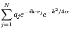 |
(233) |
 |
(234) |
We can use Eq. 229 to solve for
![]() :
:
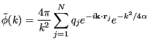
Fourier inverting
![]() gives
gives
 |
(236) |
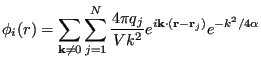 |
(237) |
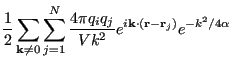
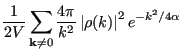
So, the total Coulombic energy due to the compensating charge distribution
is
 |
(241) |
Notice that this does indeed include a spurious self-self interaction, because
the point charge at ![]() interacts with the compensating charge
cloud also at
interacts with the compensating charge
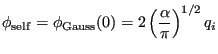
cloud also at ![]() . This self-interaction is the potential
at the center of a Gaussian charge distribution. First, we solve
Poisson's equation for the potential due to a Gaussian charge
distribution (details in F&S):
. This self-interaction is the potential
at the center of a Gaussian charge distribution. First, we solve
Poisson's equation for the potential due to a Gaussian charge
distribution (details in F&S):
 |
(242) |
| (243) |
 |
(244) |
 |
(245) |
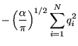
So the total self-interaction energy becomes
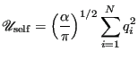 |
(246) |
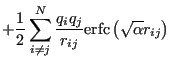
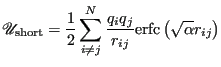
Finally, the real-space contribution of the point charge at ![]() is the
screened potential:
is the
screened potential:
| (247) |
 |
(248) |
Putting it all together:
 |
(252) |
Now, the arbitrariness left to us at this point is in a choice for the
parameter ![]() . Clearly, very small alphas make the Gaussians tighter
and therefore the compensating charge distribution less smoothly varying.
This means a Fourier series representation of
. Clearly, very small alphas make the Gaussians tighter
and therefore the compensating charge distribution less smoothly varying.
This means a Fourier series representation of
![]() with
a given number of terms is more accurate for larger
with
a given number of terms is more accurate for larger ![]() . We'll
evaluate choice of
. We'll
evaluate choice of ![]() in Sec. 6.3.
in Sec. 6.3.