A Box of Water

Here I illustrate a workflow for generating and simulating a small box of water molecules.

First, we can use `gmx insert-molecules` to generate a system with waters randomly positioned inside a box:

$ gmx insert-molecules -ci /usr/share/gromacs/top/spc216.gro \ 
  -nmol 100 -box 3 3 3 -o water_box.gro

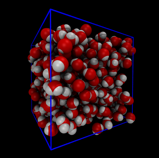
The -box switch allows us to specify a box that is 3x3x3 nm$^3$, and -ci refers to a special file containing template atomic coordinates for a single water molecule. The -nmol switch asks Gromacs to try to insert more molecules than a simple volume/density calculation would suggest (not many more can be put in). This creates the file water_box.gro, which for me contains 432 water molecules, as depicted using VMD in Fig. 32.

Figure 32: A cubic box containing 432 water molecules created using gmx insert-molecules.

Next, we need to use pdb2gmx to generate the Gromacs topology file.

$ gmx pdb2gmx -f water_box.gro -o new_water_box.gro -p topol.top

In running this command, I selected the CHARMM27 force field (which won't matter since we have nothing but water here) and the TIP3P water model. We now have the topology file and a new gromacs coordinate file (which just renames the water molecules to HOH to conform to the TIP3P naming scheme).

Now, using the minim.mdp parameter file given, we can build and run the energy minimization:

$ gmx grompp -f minim.mdp -c new_water_box.gro -p topol.top -o min.tpr
$ gmx mdrun -v -deffnm min

This will create a lot of output files that all begin with min. One of them contains all the energy-like data: min.edr. This file is binary, so the tool gmx energy is used to extract data from it:

$ gmx energy -f min.edr

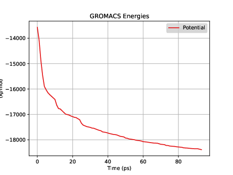
This will create energy.xvg with column-oriented time-series of whatever data is selected interactively. Fig. 33 shows what the potential energy looks like for this minimization.

Figure 33: Potential energy vs cycle in a Gromacs minimization of a box of 432 waters.

(This is a very, very minimized system; the initial water box had no overlaps really at all.) Now we can run the NVT simulation using the nvt.mdp parameter file:

$ gmx grompp -f nvt.mdp -c min.gro -p topol.top -o nvt.tpr
$ gmx mdrun -v -deffnm nvt

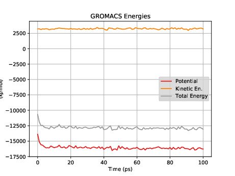
Fig. 34 shows a plot of the energies vs time for this short, short simulation.

Figure 34: Energies vs time in an NVT MD simulation (300 K) of a box of 432 water molecules.

Now let's try using the output configuration from this NVT simulation as an input for an NPT simulation.

$ gmx grompp -f npt.mdp -c nvt.gro -t nvt.cpt -p topol.top -o npt.tpr
$ gmx mdrun -v -deffnm npt

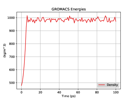
Fig. 35 shows a plot of the density vs time for this short, short simulation.

Figure 35: Density vs. time in an NPT MD simulation (1 bar, 300 K) of a box of 432 water molecules.