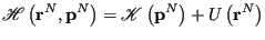
Analogous to the quasi-classical microcanonical paritition function of Eq. 6, here is the quasi-classical representation of the canonical partition function:
![$\displaystyle Q_{\rm classical} = \frac{1}{h^{dN}N!}\int \int d{\bf r}^N d{\bf p}^N \exp\left[-\beta\mathscr{H}\left({\bf r}^N,{\bf p}^N\right)\right]$](img180.png) |
(46) |
 is the Hamiltonian function which computes the energy of a point in phase space. The probability of a point in phase space is represented as
![$\displaystyle P\left({\bf r}^N,{\bf p}^N\right) = \left(Q_{\rm classical}\right)^{-1} \exp\left[-\beta\mathscr{H}\left({\bf r}^N,{\bf p}^N\right)\right].$](img182.png) |
(47) |
So, the general “sum-over-states” ensemble average of quantum statistical mechanics, first presented in Eq. 1, becomes an integral over phase space in classical statistical mechanics:
![$\displaystyle \left<G\right> = \frac{\displaystyle \int \int d{\bf r}^N d{\bf p...
...{\bf p}^N \exp\left[-\beta\mathscr{H}\left({\bf r}^N,{\bf p}^N\right)\right] },$](img183.png) |
(48) |
where
 is the value of the observable
  at phase space point
 . Before moving on, it is useful to recognize that we normally simplify this ensemble average by noting that, for a system of classical particles, the usual choice for the Hamiltonian has the form
 |
(49) |
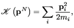
where
 is the kinetic energy, which is only a function of momenta, and
  is the potential energy, which is only a function of position. The canonical partition function,
  , can in this case be factorized:
The quantity in the left-hand braces is the ideal gas partition function, because it corresponds to the case when the potential is 0. (Note that we have multiplied and divided by  ; this is the equivalent of scaling the positions in the integration over positions.) The quantity in the right-hand braces is called the configurational partition function,
  .
.
Because the kinetic energy
has the simple form,
 |
(53) |
where  is the mass of particle
  , the integral over particle momenta can be evaluated analytically:
(We have assumed all particles have the same mass,  ; in the case
of distinct masses, this is just a product of similar factors.)
; in the case
of distinct masses, this is just a product of similar factors.)
 becomes
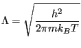
where  is the de Broglie wavelength, a quantum-mechanical property of a particle inversely proportional to its momentum (and thus inversely proportional to the square root of temperature):
 |
(58) |
As an example, for a hydrogen atom with mass 1 amu and at room temperature (298 K),
 1 Å. The de Broglie wavelength limits the precision by which a particle's position can be determined; for H atoms at room temperature, one is not permitted to specify their positions with a precision finer than about 1 ångstrom without violating the Heisenberg uncertainty principle of quantum mechanics. However, as we will see, in classical molecular simulations, we must lift this restriction, while never forgetting that this makes a classical representation of a molecule somewhat less realistic.
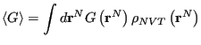
With the momentum degrees of freedom handled at finite temperature, when the observable is a function of positions only, the ensemble average becomes a configurational average:
![$\displaystyle \left<G\right> = Z^{-1}\int d{\bf r}^N \exp\left[-\beta U\left({\bf r}^N\right)\right] G\left({\bf r}^N\right).$](img208.png) |
(59) |
Note that the integration over momentum yields a factor
in both the numerator and denominator, and thus divides out. We can write this configurational average using a probability distribution,
 , as
, as
 |
(60) |
where
 |
(61) |
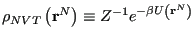
is called the “canonical probability distribution.” As pointed out on p. 15 of Frenkel & Smit [1], Eq. 59 is “the starting point for virtually all classical simulations of many-body systems”; that is, it is the starting point for almost all simulations discussed in this course.
cfa22@drexel.edu
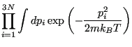
![$\displaystyle \int d{\bf p}^N \exp\left[-\beta\mathscr{K}\left({\bf p}^N\right)\right]$](img197.png)
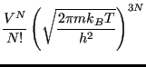
![$\displaystyle \frac{V^N}{N!h^{3N}} \int d{\bf p}^N \exp\left[-\beta\mathscr{K}\left({\bf p}^N\right)\right]$](img201.png)

![$\displaystyle \frac{1}{h^{3N}N!} \left\{\int d{\bf p}^N \exp\left[-\beta\mathsc...
... \left\{\int d{\bf r}^N \exp\left[-\beta U\left({\bf r}^N\right)\right]\right\}$](img190.png)
![$\displaystyle \left\{\frac{V^N}{h^{3N}N!} \int d{\bf p}^N \exp\left[-\beta\math...
...\{V^{-N}\int d{\bf r}^N \exp\left[-\beta U\left({\bf r}^N\right)\right]\right\}$](img191.png)